How to Make a Scatter Plot in Excel

Making a scatter plot in Excel starts with two numeric columns: x values on the left and their matching y values beside them. Select both columns, then choose Insert > Insert Scatter (X, Y) or Bubble Chart in desktop Excel for Windows.

Choose the option showing points without connecting lines for a basic plot. Each row becomes one point, and both axes represent numbers. This preserves unequal gaps between x values, which an ordinary category-based line chart does not.

1. Arrange one x-and-y pair on each row

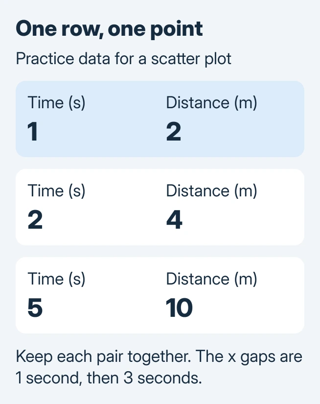
Create a heading for each column and include the units if they matter. Keep each observation's two values together. For a practice sheet, type the following invented data into A1:B4.

Time (seconds)	Distance (meters)
1	2
2	4
5	10

Microsoft documents the scatter-versus-line distinction: a scatter chart positions points using the numerical value on each axis. The gap from 2 to 5 therefore spans three time units.

Status: Excel scatter insertion and series controls checked November 2, 2026 against Microsoft guidance. The practice values are invented; no workbook was opened or chart rendered in Excel.

Do not sort just one column. Doing so can pair a time with the wrong distance while leaving a plausible-looking chart. Keep any total or summary row outside this three-observation selection.

For names such as departments or products on the horizontal axis, consider an Excel category chart instead. Scatter expects numeric x coordinates, not category labels.

2. Insert the points and label both axes

Select A1:B4, including the two headings. On Windows, open Insert, find Insert Scatter (X, Y) or Bubble Chart, and choose Scatter with markers only. Hover over an icon to read its name before selecting it.

On Excel for Mac, Microsoft's documented route uses Insert > X Y Scatter, followed by a scatter type. The controls in this guide refer to desktop Excel; do not expect every dialog to match the browser edition.

Select the resulting chart and replace its title with Distance over time. Then open Chart Design > Add Chart Element > Axis Titles. Add Primary Horizontal for time and Primary Vertical for distance.

Include seconds and meters in those axis titles. A chart title names the comparison; axis titles tell the reader what each coordinate measures.

The practice chart should contain three points. Check the point at time 5 against distance 10, then compare the other two with their source rows. A wrong point needs a data correction before visual styling.

3. Correct the series when Excel uses the wrong coordinates

Select the chart and open Chart Design > Select Data. Under Legend Entries (Series), select the plotted series and choose Edit.

Microsoft says an XY series has separate Series X values and Series Y values boxes in its series-editing reference. Check the numerical ranges independently.

For the practice sheet, the x range is A2:A4 and the y range is B2:B4. Exclude the headings from those two value boxes. Keep the same number of observations in each, then confirm the dialogs.

If the axis still behaves unexpectedly, inspect the source cells for numbers stored as text. Microsoft states that these values can cause problems, and its conversion instructions explain Convert to Number.

Convert only fields that are intended to be measurements. A product code containing digits may belong as text, and changing its type can remove meaningful leading zeros.

4. Add only the analysis the data supports

A scatter plot shows how two measurements vary together. A pattern between the points does not prove cause and effect. Keep the source and units available when sharing the workbook.

When measurements have known uncertainty, set the appropriate Excel error bars. The uncertainty amounts must come from the analysis, not an automatic styling choice.

For a chart that still plots incorrectly, give the workbook's author or Microsoft Support a small nonconfidential example. Include the two source ranges, chart type and Excel edition so they can check the same coordinates.

The Short Version

Keep numeric x-and-y pairs on the same rows, insert a marker-only scatter chart and label both axes. Check its series ranges against a known pair; equal spacing on a category axis is not the same as numerical x positioning.