How to Remove Gridlines Within an Excel Table

Excel can hide the faint grid inside a table by filling those cells, including with white. If the lines remain, they're usually cell borders or part of the table style, which need a different control.

Use the worksheet's Gridlines checkbox only when you want the grid hidden across the whole sheet. For one table, select its cells and work on their fill and borders so the surrounding worksheet keeps its grid.

Choose the area before changing its appearance

Select the table cells you want to change. Include its header and totals only if those areas should lose their lines too. For a plain rectangular list, dragging from its first cell to its last is enough.

In Excel for Windows, the Name Box beside the formula bar also lets you select an exact area. Enter a range such as B2:F20 and press Enter. Check the highlighted cells before changing their appearance.

Clicking inside an Excel table shows Table Design on Windows, or Table on Mac. A list with colors and borders may still be an ordinary cell range. You can change fills and cell borders in either.

I'd save a copy before changing the appearance of a shared report. That makes it easy to compare the finished result with the original, especially when existing colors carry meaning.

Hide the faint grid inside the selected cells

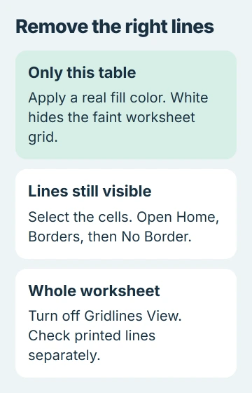
Open Home and expand Fill Color, the paint-bucket control. Choose white, or another actual fill color that suits the table. Click outside the selection to see the result clearly.

A white fill looks similar to an unfilled worksheet, but it behaves differently. Filled cells hide the worksheet's faint grid. No Fill removes that background and allows the grid to show again when worksheet gridlines are enabled.

Microsoft explains this distinction in its gridline visibility instructions. The worksheet grid can't be switched off for just a selected range; a fill hides it in those cells.

If your table has colored bands you want to keep, leave those fills in place and check the remaining lines first. A white fill would cover the bands too. If lines still show in filled cells, check the borders next.

If only part of the table changes, select the cells that still show the grid and check their fill. Empty rows just outside your selection keep their original appearance until you select and change them too.

Remove cell borders that survive a fill

Keep the intended cells selected. Open Home > Borders and choose No Border. Expand the menu to choose that command; clicking the main Borders button can repeat the last border style instead.

Click elsewhere and check the lines inside and around the table. Borders are part of the cells' formatting, so hiding the grid won't remove them. The cell border instructions explain how to remove them.

If a line remains along one edge, check the neighboring cells. That line can be a border on the cells beside your table. Select the cells on both sides of the unwanted line and apply No Border there.

Select only the extra cells you need. Removing borders from the entire worksheet can also remove useful lines around totals, input boxes and other tables you wanted to keep.

In a browser workbook, highlight the range and choose Home > Borders > No Border too. If the smaller ribbon hides the label, expand its formatting controls to find the Borders menu.

Change the table style when its design supplies the lines

For an Excel table, open Table Design > Table Styles. On Mac, look under the Table tab. Look for a preview with the fills you want and no unwanted lines between cells.

When the whole design should go, the style gallery's Clear command removes the chosen style while keeping the table. Our table-formatting guide explains how that differs from converting the data to a normal range.

Don't use Clear All just to change how the table looks. It can delete the cell contents too. Use the fill, border and table-style controls to change the appearance while keeping your values.

For a reusable design in desktop Excel, expand Table Styles and choose New Table Style. Select the relevant Table Element, then Format to set its Border and Fill choices. Inspect the design preview, then apply the finished style.

A custom style helps when you want future rows to keep the same design. For a report you're finishing once, a suitable built-in style is usually quicker.

Hide the grid across the worksheet when that's the goal

In Excel for Windows, open View and clear Gridlines in the Show group. Excel for the web offers the checkbox on View too. Click a cell first if another selected object is keeping ribbon controls unavailable.

On Mac, use Page Layout > Gridlines and clear View. This controls the grid you see on screen across the selected worksheet, including cells outside your selection.

Check that only the intended worksheet tabs are selected. If several are grouped, right-click a selected tab and choose Ungroup Sheets before continuing with other formatting work.

The grid should disappear from unfilled cells across that sheet. Any lines left are other formatting or guides. Dashed lines across the page come from the separate page-break display setting.

Check the printed result and get help for stubborn formatting

Open File > Print and check the preview. In desktop Excel, the checkbox at Page Layout > Sheet Options > Gridlines > Print controls printed gridlines. Clear Print if you don't want them on paper.

Excel for the web doesn't print ordinary worksheet gridlines. Lines in its printout come from formatting such as cell borders. Return to the selected cells and remove the borders responsible.

If the lines keep returning, save a copy and note whether a table style or an edit brings them back. Remove private data from a small example, then send it to Microsoft support with your Excel version.

The Short Version

For one table, apply a real fill and remove unwanted cell borders. Keep No Fill for cells that should show the worksheet grid. Use the worksheet-wide Gridlines control only for a whole-sheet change, then check print preview separately.

Checked November 5, 2026.