How to Combine Excel Spreadsheets Into One Table

Combining Excel spreadsheets into one list is easiest with Power Query's Append Queries command. Prepare matching column headings, load each source as a query and append their rows. For totals instead of a combined list, use Consolidate.

Use desktop Excel on Windows for these steps. Your source tables stay separate from the combined result. This suits monthly lists with the same fields, such as two sheets containing Date, Item and Amount.

1. Decide whether the result needs rows or totals

Appending keeps each record: three purchases from one sheet and two from another become five purchases in one table. Consolidating adds up matching values or summarizes them another way.

Microsoft says to choose the combination method by the result. A summary can look tidy while leaving out the individual records you needed.

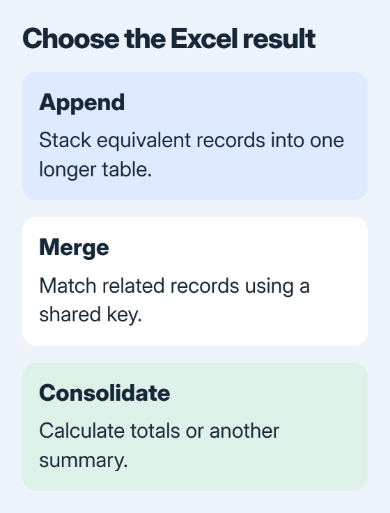
Merge joins related tables using matching values, such as a product code. Use Append when your lists contain the same kinds of records and you want to stack them one after another.

To keep several complete sheets as separate tabs in one workbook, use the worksheet-copy procedure instead. Appending data builds one result table; it doesn't copy every sheet's layout and objects.

2. Give the source tables matching column headings

Keep a single header row on each list. Use the same names for equivalent fields, such as Date, Item and Amount. Remove title rows or totals from the selected data range when they aren't actual records.

Select the first list and press Ctrl + T. Check the selected range, turn on My table has headers, then confirm. Repeat for the second list. These are Excel tables, rather than ranges that only look formatted.

Use Table Design > Table Name to name each table, such as JanuaryData and FebruaryData. Different names make it easier to choose the right sources when the Append dialog opens.

The table creation instructions explain selecting the range and identifying headers. Check both the first record and the last one so a total isn't included by mistake.

The append reference explains that columns match by header name, rather than their position. If one list says Amount and another says Cost, the result can contain two separate fields.

Give columns that contain the same kind of data matching headings. Keep different fields separate: a shipping cost and an order total mean different things, even though both contain numbers.

3. Create a query for each source table

Click inside the first table and choose Data > From Table/Range. Excel opens the Power Query Editor in a separate window. A query stores the steps used to read and reshape your source data.

Check that the first row became the headings and that the preview includes the records you expect. Check the data types beside the headings, such as date, number or text, especially for amounts and codes that need leading zeros.

Choose Home > Close & Load > Close & Load To, select Only Create Connection in the Import Data dialog, then confirm. Other queries can now use this source without adding an extra worksheet for its results.

Repeat for the second table. The query loading guide explains switching between the worksheet and editor, along with the Load To choices.

If Close & Load To isn't available on the first import, finish Close & Load. Then open Data > Queries & Connections, right-click the query and choose Load To to change where its results load.

Both sources should now appear under Queries & Connections. Give the queries clear names if their default names are confusing. Keep your original tables; the combined query reads them again when you refresh it.

4. Append the sources into a new query

Double-click the first query in Queries & Connections to reopen it in the editor. Open the menu beside Home > Append Queries and choose Append Queries as New.

Choose Two tables and check both source selections. For more lists, choose Three or more tables and add the required queries to Tables to append. Put them in the order you want the sources appended.

Select OK and check the new query's preview. The first source's records should appear before the second source's records. Columns with matching headings should become one column, rather than two with similar names.

The as New choice keeps your two source queries and creates a third for the combined result. Name it CombinedData or something equally clear so you'll recognize it later.

Choose Home > Close & Load to load the result into a worksheet. If Excel asks for a destination, choose a new worksheet for this first check. That makes the combined output easy to compare with its inputs.

5. Check the rows before relying on the result

Count the records in each source, leaving out headers and totals. In the example with three January records and two February records, you should get five combined records. Check any difference before using the table in a report.

Check a record from each source, including its date, description and amount. An unexpected extra column with empty cells often means a heading didn't match. Fix the source heading and refresh, rather than editing the output by hand.

Append keeps duplicate records unless you add a separate removal step. If the same transaction appears in both inputs, it can appear twice in the result. Use the duplicate-removal guide only after deciding which fields identify a duplicate.

For lists stored in many separate files, the folder import procedure provides a different starting point. It suits files with matching structure collected in one folder.

6. Refresh when the source lists change

Enter new records in the original source tables. Then choose Data > Refresh All and wait for the combined output to update. The connection refresh guide explains retrieving updated source data.

Don't use the query's output as your permanent data-entry sheet. Refreshing rebuilds it from your sources and saved steps. Make corrections in the source table or in the query step that should produce them.

If the tables still won't combine, note your Excel edition, query name and error. Make a small example with matching headings and records you can safely share, then ask whoever maintains the workbook or Microsoft Support for help.

The Short Version

Use Append for one list of records and Consolidate for totals. Turn the source ranges into tables, create their queries, choose Append Queries as New and check the resulting rows. Update the sources and refresh the result afterward.

Checked November 5, 2026.