
A trendline in Excel goes on a chart's data series. Select the points or line, then choose Chart Design > Add Chart Element > Trendline in desktop Excel. Start with Linear for a straight-line pattern.
With several series, select the one you want before adding its trendline. For paired numeric measurements, an XY scatter chart keeps the actual spacing between horizontal values. Check the chart type before drawing conclusions.
Prepare the chart before adding the fit
Put the horizontal measurements in one column and their matching results in the next. Each row should represent one pair. Leave totals, notes, and unrelated measurements out of your selection.
For a small example, enter 1, 2, 3, 4, 5 in A2:A6 and 3, 5, 7, 9, 11 in B2:B6. Add headings in row 1, select the range, and insert a scatter chart with markers.
Those example points follow y = 2x + 1. They make it easy to check whether Excel is using the columns you intended. Replace them with your real observations after you understand what the selected series represents.
The Excel scatter chart steps cover the initial chart. A line chart can suit categories or regularly spaced periods, but it doesn't treat every horizontal label as a numeric x-coordinate in the same way.
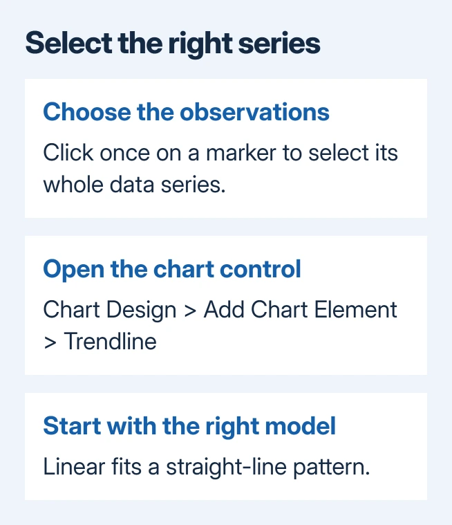
Click a marker once to select its whole series. A second click can select only one point, which isn't the selection you want for a series trendline. Check that the other markers in that series are selected too.
Add the trendline in Windows desktop Excel
With the intended series selected, open Chart Design > Add Chart Element > Trendline. Choose Linear, or select More Trendline Options when you need a different model or additional settings.
Microsoft's trendline instructions also show the Chart Elements button beside a selected chart in Windows. Open it and use Trendline to add the fit.
If Excel asks which series to use, select the named series that contains the measurements you want to analyze. Check its name against the chart legend and the worksheet headings before confirming your choice.
A new line should appear across that series. Select the line to open its formatting options. Changing its color or thickness makes it easier to tell apart from your data points, but doesn't change the calculation behind it.
I'd name a series before adding several trendlines. Temperature and Pressure are much easier to distinguish in a selection list than Series1 and Series2, especially after the chart has been copied into a report.
Use the Mac or browser controls for that version
In Excel for Mac, choose View > Normal, select the chart's data series, then open Chart Design > Add Chart Element > Trendline. Pick the model or choose More Trendline Options for the detailed controls.
To remove it on Mac, use Chart Design > Add Chart Element > Trendline > None. Selecting the trendline itself and pressing Delete also removes that chart element, so check the selection before pressing the key.
In the web editor, clicking the chart exposes its Chart ribbon tab. Open Format, expand the required Series, and customize its Trendline settings. Its switch shows or hides the trendline.
The browser has its own chart formatting controls; it doesn't use the Windows floating Chart Elements button. If the workbook is read-only, ask the owner for editing access before trying to change chart settings.
These instructions apply to supported Excel desktop releases and Microsoft 365. If your edition's interface differs, open its chart-formatting pane and check that you've selected the series you want, rather than the chart background.
Pick a model that answers the question
Linear fits a straight line to the data. Moving Average smooths rises and falls by averaging neighboring points. Its Period setting controls how many points go into each average, so changing it changes the pattern you see.
Exponential, Logarithmic, Polynomial, and Power describe other shapes. They aren't just different visual styles. Choose one that suits your measurements and analysis, rather than the one with the neatest curve.
Some models need particular input values. For example, exponential and power fits have restrictions involving zero or negative values. An option can be grayed out because of the values in that series, even when Excel is working normally.
Check the trendline model requirements before changing the original observations to make a model available. A real zero shouldn't disappear simply to permit a particular curve.
If the chart needs uncertainty around the measurements, add the appropriate Excel error bars separately. A trendline shows a fitted pattern; it doesn't tell you how uncertain the measurements are.
Show the equation carefully and limit the forecast
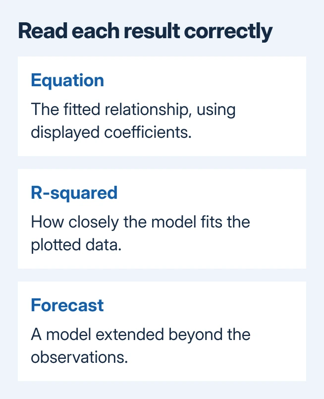
For a model that offers them, enable Display Equation on chart and Display R-squared value on chart in the trendline's formatting options.
R-squared describes how closely the model fits your data points. A close fit doesn't show that one variable causes another.
The sample points should produce a slope of 2 and an intercept of 1 for a linear fit. If the equation differs, check which values the chart uses before choosing another model.
Displayed equations can be rounded. If the equation's numbers give a different result from the chart, show more decimal places in the equation label's number formatting. The equation precision fix addresses that specific issue.
The Forward and Backward fields extend a supported trendline beyond the data points. Keep those extensions modest and label them clearly. The extended part shows what the model predicts, not new measurements.
Leave Set Intercept unchanged unless the analysis requires it. Forcing the line through zero changes the fit. Beginning with version 2005, Excel also changed R-squared calculations for zero-intercept linear trendlines.
If the command stays unavailable, check the chart type, selected series, and model restrictions. If all are supported, send Microsoft Support a sample workbook, your Excel version, and the name of the grayed-out control.
The Short Version
Choose your chart series before adding the trendline and selecting its model. Use the Mac or web controls for that edition. Check the equation's precision and label any forecast as a projection beyond the observed data.
Checked November 9, 2026.

Isaac Smith is the founder and editor of PC Glance, a website that covers computers, laptops, and technology. He is a tech enthusiast and a computer geek who loves to share his insights and help his readers make smart choices when buying tech gadgets or laptops. He is always curious and updated about the latest tech trends.