

Excel shows a spill error where your results should be, across the next few cells. The formula itself looks right.
I'll explain how to read the reason attached to #SPILL! and fix that specific problem. Don't begin by clearing the whole worksheet.
Select the error before changing your formula
Click the cell showing #SPILL!, then open its error alert. Microsoft says Excel can report different causes, including occupied cells, a table formula, merged cells or an output range that cannot fit.
Its SPILL troubleshooting page explains each message. The outlined area that appears when you select the formula shows where Excel wants to place the results.
Status: Microsoft's dynamic-array and SPILL guidance checked 18 October 2026. These fixes concern spilled formulas; the exact error reason decides which change you need.
Keep your data while locating the obstruction. I would save a copy before reorganizing a workbook that other people also use.
Occupied range: move the blocking entry
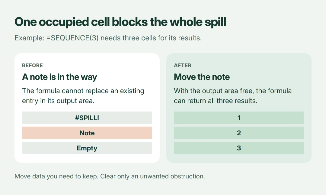
For Spill range isn't blank, use Select Obstructing Cells from the error alert. Microsoft documents this command to take you directly to the cells preventing the output.
Move an entry you need to keep, or clear only the unwanted contents. Once the required space is empty, the formula can return its results automatically.
Don't judge a cell by its appearance alone, because what you see can differ from the value or formula stored inside it.
Select it and read the formula bar before deciding it contains nothing, particularly in a workbook with formulas that display blank results.
This repair gives your formula an empty destination for every value it needs to return. Changing the formula's font or widening the column won't remove a blocking value.
Merged cells: separate them or move the formula
Microsoft states that a spilled array cannot expand into merged cells. Your options are to unmerge the affected cells or place the formula somewhere with an uninterrupted output area.
On the Home tab, open the Merge & Center menu and choose Unmerge Cells for the affected selection. If the merged heading belongs to a report layout, moving the formula may preserve that layout more neatly.
Merging also causes other worksheet problems. Our AutoFit row-height explanation covers the separate case where wrapped text won't fit correctly.
Table formula: put the result outside the table
Spilled formulas cannot occupy an Excel table's calculated column. Microsoft's dynamic-array guidance distinguishes the source data from the place where results appear.
Your source data can stay in a table. Put the spilling formula in ordinary worksheet cells outside it, with enough free cells for the returned values.
In Excel for Windows, another supported choice is converting the table to an ordinary range through Table Design > Convert to Range. I would use that only when you don't need the table's behavior anymore.
A table reference isn't inherently wrong. It is the location of the spilling formula that matters in this case.
Worksheet edge: narrow the requested results
A whole-column lookup can ask Excel to return more rows than fit from the formula's starting cell. Microsoft's example places =VLOOKUP(A:A,A:C,2,FALSE) in E2 and requests an entire column of answers.
The worksheet has 1,048,576 rows. Starting those results in row 2 makes the last result extend past the sheet, even if every visible cell looks empty.
If you only need six lookup values, Microsoft's bounded example is =VLOOKUP(A2:A7,A:C,2,FALSE). Change those addresses to match your real data rather than copying them blindly.
Need one answer per row instead? Use a single lookup cell, such as =VLOOKUP(A2,A:C,2,FALSE), and fill the formula down for the rows you need.
The @ operator can also request a single intersecting value, but that changes the intended result. Don't add it merely to hide an error when you actually need the complete list.
Indeterminate size: stop changing the output dimensions
An array whose size changes during recalculation may never settle. Microsoft illustrates this with =SEQUENCE(RANDBETWEEN(1,1000)), where the random number decides how many rows the formula needs.
Give the row count a stable value or a stable cell reference. Then the requested area stops resizing between calculation passes and Excel can place the result.
Not every changing calculation causes this error. The relevant problem is an unstable output size, so don't remove every date function from your workbook.
Out of memory: reduce the array first
For the memory reason attached to #SPILL!, Microsoft's advice is a smaller array or range. Replace unnecessary whole-column inputs with the rows your calculation actually needs.
For an unrecognized reason, check the function's required arguments against its documentation. If your cell displays the formula as text instead of an error, use our formula-display checks.
That text-display symptom follows a different set of checks from the spill error you're seeing here. Reinstalling Office won't free an occupied spill cell or turn a table column into a suitable output area.
The Short Version
Read the error alert first. Move blocking contents, unmerge the output cells, or move a table formula into ordinary cells. Reduce oversized ranges and keep array dimensions stable when Excel reports those causes.
Where to Next
Which reason appears beside your #SPILL! cell, and what formula are you using? Tell me the reason and a version of the formula with private workbook names removed. I can then see whether the output needs space or a different shape.

Isaac Smith is the founder and editor of PC Glance, a website that covers computers, laptops, and technology. He is a tech enthusiast and a computer geek who loves to share his insights and help his readers make smart choices when buying tech gadgets or laptops. He is always curious and updated about the latest tech trends.