How to Make a Bar Chart in Excel

A horizontal bar chart in Excel starts with category names and their numeric values. Select both columns, then choose a Clustered Bar chart. This keeps long labels readable on the left and compares values along the horizontal scale.

For a simple comparison, start with one value per category. Stacked bars answer a different question: how several components contribute to each category's total.

Arrange the labels and values before inserting the chart

Enter a heading such as Item in A1 and Orders in B1. Put Keyboard, Mouse and Headset in A2:A4, with the example counts 8, 12 and 6 in B2:B4. Select A1:B4.

Microsoft documents rows or columns as suitable source data for a bar chart. Including the headings gives Excel the category and series context along with the values.

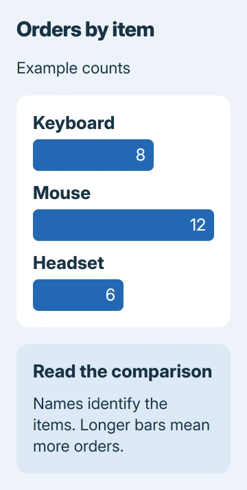
Status: Excel chart creation, bar types and category-order controls checked against Microsoft instructions November 3, 2026. The pictured counts are invented example data.

Keep each label beside its matching number. Leave any grand-total row outside this selection unless the total itself should be plotted as another category; otherwise it produces an extra bar that changes the comparison.

For pairs of numeric measurements, such as height against weight, use an Excel scatter plot instead. The bar chart here compares named groups, not pairs of numeric coordinates.

Insert a clustered horizontal bar chart

In Excel for Windows, choose Insert > Recommended Charts > All Charts. Select Bar, choose Clustered Bar, inspect the preview and select OK. The chart appears on the worksheet.

On Mac, open Insert, select the bar chart type and double-click the chart you want. In Excel for the web, use Insert > Charts and select the bar type from the available gallery.

Microsoft says bar charts suit long category labels. Their bars run horizontally. A Column chart turns the comparison upright, so check the preview before accepting it.

For the example, Mouse should have the longest bar at 12, Keyboard should show 8 and Headset should show 6. A chart with three equally sized bars does not represent those values correctly.

If the wrong cells were included, select the chart and use Chart Design > Select Data in desktop Excel. In the web version, right-click the chart and choose Select Data to change its source range in the task pane.

Use stacked bars only when the parts matter

A clustered chart puts separate series beside one another within each category. For example, two count columns could compare this month's orders with last month's for each item.

A Stacked Bar combines the series within each bar to show their contribution to a total. A 100% Stacked Bar compares their proportions instead, so bars have the same overall length even when totals differ.

Microsoft states these distinctions in its chart-type guidance. Choose clustered bars when the reader needs to compare individual counts directly; choose stacking when the relationship between parts is the point.

Fix the order and make the result readable

Excel can display categories in the opposite vertical order from the worksheet. In desktop Excel, select the category labels and open Format > Format Selection. Under Axis Options, select Categories in reverse order if needed.

Microsoft's plotting-order instructions document that control. It changes the displayed order without requiring the source rows to be rearranged.

Give the chart a title that identifies the measure, such as Orders by Item. In desktop Excel, select it and use Chart Design > Add Chart Element for Chart Title or Data Labels. Enlarge the chart if category names are cramped.

For other chart layouts and source-selection questions, the general Excel chart guide covers the wider workflow. Avoid adding decorative effects that make the bar lengths harder to compare.

If the chart still misrepresents the table, compare each category and value with its selected cells. For persistent problems, ask Microsoft Support to inspect a reduced workbook containing made-up data.

The Short Version

Select category names with their numbers and insert a Clustered Bar chart. Check the longest bar against the largest value, adjust category order if needed, and add a clear title and readable labels.