How to Color Every Other Row in Excel

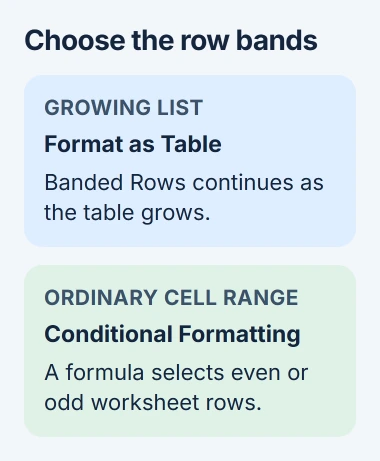
Color every other row in Excel with Home > Format as Table and a banded table style. For a worksheet that must stay a normal cell range, use a conditional formatting formula instead.

I'd choose the table for a list that keeps growing. Its alternating colors continue when rows are added or removed. The formula gives you more control over which worksheet rows get a color.

Use a banded table for a growing list

In desktop Excel, select the cells in your list, including its header row when it has one. Choose Home > Format as Table, then pick a style with alternating light and unfilled rows.

Check the cell range in the dialog. Select My table has headers only if your selection already includes the column names, then choose OK. The list becomes an Excel table, with its own style and filtering controls.

Click a cell in the new table and open Table Design. In Table Style Options, check Banded Rows. If Banded Columns is also selected and you only want horizontal bands, clear that option.

The colors should alternate across the selected table so you can follow each record across several columns. The header can have a stronger color of its own; it doesn't have to match the rows of data.

Microsoft's alternating-shading instructions describe both table banding and formula rules. The table method is useful when you also want its sorting and filtering controls.

When you add data, check that the new row is part of the table. Don't leave a blank gap between it and the existing list. A row outside the table won't get the table's formatting.

Keep an ordinary range with a formula rule

Use this method in desktop Excel for Windows if a table would get in the way of your worksheet layout. Select only the cells you want to shade, such as A2:D20, leaving your headings out.

Open Home > Conditional Formatting > New Rule. Choose Use a formula to determine which cells to format, then enter this formula in the rule box:

=MOD(ROW(),2)=0

Choose Format > Fill and pick a light background color. Select OK to return to the rule, check the preview, then select OK again to apply it.

Conditional formatting tells Excel to change a cell's appearance when a condition is met. Here, ROW() gives the worksheet row number. MOD gives the remainder after division, so this rule matches even-numbered rows.

In A2:D20, rows 2, 4 and 6 get the color, continuing through row 20. Rows 3 and 5 don't. Every selected cell on a matching row gets that background, so the band covers all four selected columns.

The formula belongs in the formatting rule, not in a worksheet cell. Typing it into A2 would replace that cell's data and return a formula result instead of coloring your list.

If Excel reports a formula error, check the punctuation and the separator your regional settings use. Some installations need semicolons between the parts of a function; use =MOD(ROW();2)=0 there.

Choose whether the first data row gets a color

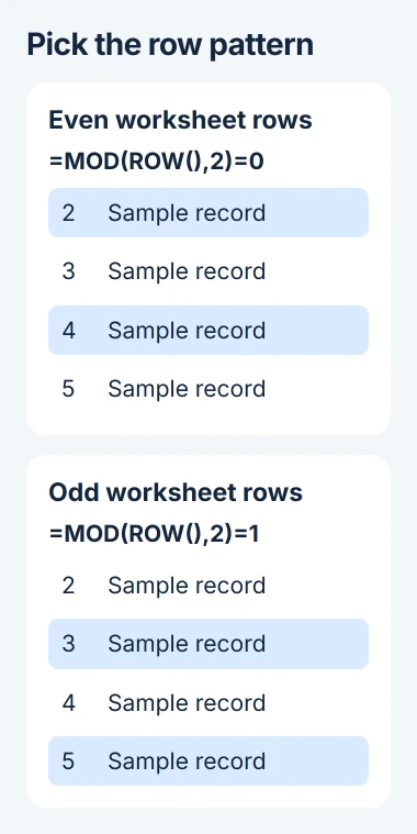
The even-row rule uses worksheet row numbers. It doesn't count the first row of your selection as row one. That's why a list starting on row 3 begins without a fill when you use the formula ending in =0.

To shade odd worksheet rows instead, use:

=MOD(ROW(),2)=1

For a list beginning at A3, that shades row 3, leaves row 4 unfilled, and shades row 5. Both formulas alternate the colors; choose the one that starts the way you want.

This matters when a title, note or heading takes up the first few rows. Look at the row numbers along the worksheet edge rather than counting records from the top of your list.

Neither formula depends on the text or numbers stored in those cells. Changing a customer's name or an amount won't change whether its worksheet row number is odd or even.

If unwanted empty records are making the list hard to follow, remove the blank rows before choosing the final appearance. Shading makes an empty row easier to see; it doesn't remove it.

Extend or adjust the rule from Manage Rules

Click a cell in the formatted area and choose Home > Conditional Formatting > Manage Rules. If you can't see the rule, change the list to This Worksheet to show rules across the sheet.

Check the Applies to field. For the example, it should cover =$A$2:$D$20. If new records extend to row 35, expand the range to =$A$2:$D$35, then apply the change.

Even with the right formula, an incorrect Applies to range can color just one column or leave later records plain. Check that range before replacing a formula that may already work.

To change the shade, edit the rule, choose Format, and select another fill. Check that you can still read your text. Black text usually stays clearer against a pale fill than a dark band.

If another conditional rule also sets a fill color, check which rules apply to those cells and their order of priority. Change only your row-banding rule, especially when other colors mark overdue or unusual values.

Remove the bands without deleting the list

For a table, clear Banded Rows under Table Design to remove the alternating row effect. Other parts of the style, including its header formatting, can remain.

For a formula rule, select its entry in Manage Rules and choose Delete Rule. That removes the condition while leaving cell values in place. Avoid clearing every rule if your sheet uses other useful highlights.

Converting a table to a range is a separate choice. The table-to-range instructions explain that change. Its existing appearance can remain, but future rows lose automatic table banding.

If the colors still look wrong, check whether someone also filled those cells manually. A row-banding rule and a manually chosen fill are separate, so removing one doesn't necessarily remove the other.

When the formatting controls aren't available

These formula steps use desktop Excel for Windows. If your edition has a different rule editor, use its table-banding controls or open that workbook in the Windows desktop app for these steps.

For a protected or shared work template, ask the owner whether you can change the formatting. Tell them which cells need bands and whether you want a table or ordinary range. Don't change the layout to get around a restriction.

The Short Version

Use Format as Table and Banded Rows for a list that grows. For an ordinary range, create a formula rule using MOD and ROW. Check even versus odd row numbers and expand Applies to when the list gets longer.

Checked November 5, 2026.