How to Reference Another Sheet in Excel

To reference another sheet in Excel, enter a formula such as =Sheet2!B2. The sheet name comes before the exclamation point and the cell address after it. When the source changes, the linked result updates as Excel calculates.

The easiest way to build that formula is to type =, click the source sheet's tab, then click its cell and press Enter. Excel writes the sheet name for you, including the punctuation needed for names with spaces.

Build the reference by clicking the source cell

Open the workbook and choose a destination cell for the linked value. This is the destination cell, such as B2 on a sheet named Summary. Start in that cell so you don't replace the original information.

Type =, then click the source worksheet's tab. Click the cell containing the value you want and press Enter. The destination should show that value, while its formula bar shows a reference to the source sheet.

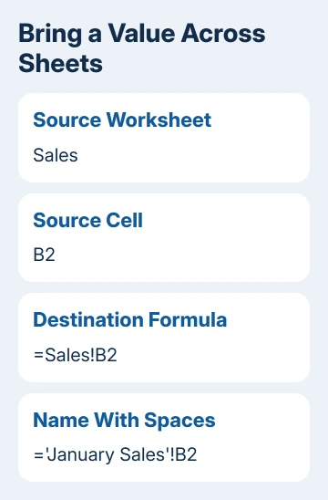
For example, if the source tab is Sales and its value is in B2, the formula is =Sales!B2. B2 in that formula refers to the Sales sheet, even if you put the formula in B2 on Summary.

Microsoft says to use this sheet-name structure in its cell-reference instructions. The formula links a cell without copying the source worksheet.

I'd build the first reference by clicking rather than typing a long sheet name. It avoids a misspelled tab name and helps you confirm the worksheet selection before copying the formula elsewhere.

Put single quotes around sheet names with spaces

For a sheet called January Sales, use ='January Sales'!B2. The single quotes enclose the sheet name; the exclamation point and cell address stay outside them.

Typing =January Sales!B2 leaves Excel without the correct sheet-name punctuation. Clicking the worksheet while building the formula is simpler because Excel adds the single quotes for you.

Use the actual tab name, including spaces and punctuation. A label typed into the top row of a worksheet isn't its tab name. Check the name on the source sheet's tab.

For #NAME?, check spelling and quotes before changing workbook settings. The Excel name-error checks explain how an unrecognized name differs from a missing reference.

A reference that works while you click through the sheets but fails when typed usually has a mistake in how the formula is written. Compare the typed version with one Excel creates from a direct cell selection.

Add or average a range from another worksheet

A reference can supply a whole range to a calculation. To add Sales cells B2 through B10, enter =SUM(Sales!B2:B10). To calculate their average, use =AVERAGE(Sales!B2:B10).

The colon includes all the cells between the two addresses. B2:B10 covers nine cells, starting with B2 and ending with B10. Check the selected rows so a total doesn't accidentally include its own result or an unrelated figure.

For a tab with spaces, keep the same quoting rule: =SUM('January Sales'!B2:B10). The sheet name appears once because the complete range belongs to that worksheet.

Build a longer formula up to the point where you need the reference, click the source tab, and select the range. Finish the closing parenthesis and press Enter. Check the formula bar if you aren't sure which range Excel inserted.

A total that refers back to itself through another sheet creates a loop. Use the circular-reference tracing steps to follow the cells that feed each other.

Choose whether the reference should move when copied

Excel normally adjusts a reference as you copy a formula. Copying =Sales!B2 down one row changes it to =Sales!B3. That's useful when you're pulling a list of values from matching source rows.

For one fixed source cell, use =Sales!$B$2. The dollar signs hold both the column and row in place. Copying that formula elsewhere keeps it tied to Sales B2.

Mixed references hold only one part: $B2 fixes column B while allowing the row to change, and B$2 fixes row 2 while allowing the column to change. Choose them only when that matches the layout you're copying across.

The reference-type instructions explain these changes. Typing dollar signs also avoids differences in laptop and Mac shortcuts.

After filling a row or column, inspect the first copied formula and one farther along. A plausible result can still come from the wrong source row, especially when adjacent cells contain similar numbers.

Keep another sheet separate from another workbook

These formulas link worksheets inside one workbook. A reference to a different file has extra workbook information, and can also include a file path. Don't add a file name to an ordinary same-workbook reference.

For a simple summary, keep the source and destination tabs in the same workbook when practical. That avoids needing another file's location just to retrieve a single value.

Moving a sheet or deleting a source changes more than its visual position in your tab list. Before removing a source sheet, review formulas that depend on it and save a copy of the workbook if the information matters.

For #REF! after deleting cells, undo the deletion if it just happened, or edit the formula to use the intended existing cell. Replacing the error with a random number hides the broken calculation.

Ask the workbook's author which tab and cell should supply a missing value. If a simple example still won't work, send Microsoft Support your Excel version, formula and sample tab names after removing private information.

The Short Version

Type an equals sign, click the source sheet and cell, then press Enter. Use single quotes around sheet names with spaces. Add dollar signs when copied formulas must keep the same source, and check the formula bar after filling a range.

Checked November 9, 2026.