

Excel can copy nonblank values into a second column without gaps. In Microsoft 365, Excel 2021 or Excel 2024, use FILTER in B1 to collect A1:A10. Its results expand down column B and update with the source.
First, decide whether you want a list without gaps or each result beside its original cell. Keeping the original rows needs a different formula. That choice prevents a result that looks right but separates values from their records.
In this guide
Build a compact list with FILTER
Suppose A1:A10 contains five numbers and five empty cells. Click B1, enter the formula, and press Enter:
=FILTER(A1:A10,A1:A10<>"","")The first part is the source range. The second part keeps values that aren't blank or empty text. The final pair of quotes tells Excel to return empty text when no source cell meets the condition.
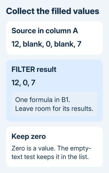
Enter the formula only in B1. FILTER returns several results from that one cell, a behavior called spilling. Don't drag the formula down through the result area as you would with an ordinary one-result formula.
Change the range to match your worksheet. If row 1 contains a heading and the data starts in A2, use A2:A11 and place the formula in B2. Keep the source and condition ranges the same size.
The output keeps the source order and repeated values. It doesn't sort the numbers or remove duplicates. A compact list is simply the filled entries with the gaps removed from the result, while column A stays intact.
Microsoft's FILTER function instructions list the supported editions. If Excel shows #NAME?, check the app's edition and the formula spelling before changing the workbook.
Keep the original rows when alignment matters
Use this formula in B1 when each result must remain next to the matching source cell:
=IF(A1<>"",A1,"")Fill that formula down through B10. A filled source cell returns its value; an empty source cell leaves an empty-looking result on the same row. The gaps remain so each result stays on its original row.
This is the right layout when column A belongs to records containing names, dates or other fields. Compressing only the numbers would detach them from those neighboring details. Filter whole records if those fields need to travel together.
For a different result when a cell contains something, replace the second A1 with the calculation or value you need. The IF not blank guide explains how that test differs from checking whether a cell has never held a value.
This one-step IF formula won't build a compact list:
=IF(A1="",A2,A1)It looks only one cell ahead. Two or more consecutive blanks can still return an empty result, and filling it down can repeat a value.
That one-step formula appeared in the original discussion, but it doesn't solve the full task of collecting every filled entry without gaps. FILTER checks the whole selected range in one calculation.
Decide what should count as blank
The nonblank condition excludes truly empty cells and formulas that return empty text. A zero stays in the output because zero is a value. That's normally useful when the list contains measurements or quantities.
A cell containing a space also stays in the output. It may look blank, but Excel sees a character. Select a suspicious source cell. Read its contents using the formula bar, then decide whether the selection rule needs changing.
For a list that should contain numbers only, use this version:
=FILTER(A1:A10,ISNUMBER(A1:A10),"")That excludes text, including numbers imported as text. A number can therefore look correct but be omitted. Choose this version when you want only cells Excel stores as numbers, rather than every nonblank entry.
An error in a source cell can make the nonblank check return an error too. Correct it or decide how the workbook should handle it before adding a function that hides it. A missing value and an invalid calculation need different treatment.
Add sorting when the values need a new order
I'd keep FILTER alone when the source order matters. For an ascending list, put SORT around FILTER:
=SORT(FILTER(A1:A10,A1:A10<>"",""))This changes the order of the output, leaving the source range alone. For a simple numeric list, the smallest number appears first. Repeated numbers remain repeated because sorting doesn't remove them.
If your data mixes text and numeric cells, check the result carefully. Numbers stored as text don't behave like numeric values in every operation. Convert those source entries to numbers when you need them all sorted numerically.
The original asker later requested values in order without blank spaces. Sorting a filtered list answers that additional requirement; sorting alone still leaves blank entries to handle.
For a task that actually requires deleting empty worksheet rows, use the blank-row removal guide. Creating a separate result column doesn't delete or move any source rows.
Clear the output area when #SPILL! appears
Click the formula cell if Excel shows #SPILL!. Check the cells where its results need to appear. Text, another formula or a merged cell can prevent Excel from placing the full list there.
Move the formula to an empty area or clear only the cells you intended to use for its results. An empty-looking formula in that area still occupies a cell. Keep the original data separate from the space reserved for output.
Place the spilling formula outside an Excel table. A table can supply the source data, but the expanding result needs space in the worksheet outside the table. Select the top formula cell whenever you need to edit the formula.
If a spill error continues, use the error indicator beside the formula for its stated reason. Send that reason and a small sample range to your workbook owner rather than replacing the formula with a long expression that hides the problem.
Use a filtered copy in older Excel editions
Excel 2016 and Excel 2019 don't have FILTER. For a one-time compact list, select the source with its heading and choose Data > Filter. Open the column's filter menu and clear (Blanks).
Select the filtered data without the heading. On Windows, choose Home > Find & Select > Go To Special > Visible cells only > OK. Copy the selection and paste into a separate empty column. Restore the source filter when finished.
This creates a copied list rather than a live formula result. Repeat the copy when the source changes. For an older workbook that needs automatic updates, ask its owner for a solution that fits its Excel version and layout.
The Short Version
Use FILTER for a live list without gaps, IF to keep the original rows, and SORT around FILTER when the values need ordering. Leave room for the results, keep zero when it matters, and use a filtered copy in older Excel editions.
Checked November 16, 2026.