Find the Range in Excel With MAX and MIN

To find the statistical range in Excel, subtract the smallest value from the largest: =MAX(A2:A6)-MIN(A2:A6). Replace A2:A6 with your numbers, and put the formula in a separate cell outside that group.

This returns the distance between the two extremes. It doesn't count the cells or calculate their average. For a filtered list, you'll need a different formula if only the visible rows should count.

Enter a formula for the highest minus the lowest

Click an empty result cell, type the formula and press Enter. Both functions must use the same measurements. MAX finds the largest number and MIN finds the smallest. Subtracting them gives you the difference.

For a small practice example, enter 12, 18, 25, 30, 15 in A2 through A6, with one number in each cell. Type the formula in C2. The expected result is 18, because 30 minus 12 is 18.

=MAX(A2:A6)-MIN(A2:A6)

Microsoft's maximum and minimum instructions show how to use each function. Subtracting their results gives you the range without sorting your measurements.

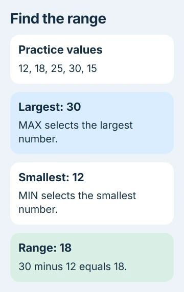
Keep a label such as Range beside C2. Include the units too: measurements in minutes give a range in minutes. Without a label, it's easy to mistake the result for the total or the largest measurement.

I'd check the two extremes separately the first time. Enter =MAX(A2:A6) in another blank cell and =MIN(A2:A6) beside it. Seeing 30 and 12 makes an unexpected range easier to trace.

Select the observations you actually mean to measure

For your own data, replace the example address with the cells containing your measurements. B2:B101 includes both endpoints and every cell between them. The colon joins the first and last cell in that selection.

Leave totals, averages and earlier results outside the selected cells. If a total is larger than every observation, MAX can select that total and give a mathematically correct answer to the wrong question.

Keep the result outside the cells it measures too. If the formula includes its own cell, you get a circular reference: the formula needs its own answer to calculate. Put it in a separate summary cell instead.

For measurements in two groups, put the combined result in F2 and give both selections to each function. This example uses A2:A6 and D2:D6, keeping the output outside both groups.

=MAX(A2:A6,D2:D6)-MIN(A2:A6,D2:D6)

Use the separator your Excel installation expects. Some regional settings use semicolons between the groups inside a function. If Excel rejects the formula, check that separator even when the cell addresses look right.

If you copy the result formula elsewhere, check whether its addresses moved. The Excel formula-copying guide explains when relative references should move and when dollar signs should keep an input group fixed.

Check numbers, blanks and zeros before trusting the result

When MAX and MIN read cells, they use numbers and ignore text, empty cells and logical values such as TRUE and FALSE. A blank and a numeric zero affect the result differently: zero counts and can become the minimum.

Don't replace missing measurements with zero just to fill the column. If your actual values run from 12 to 30, adding a zero expands the reported range from 18 to 30 even though no new measurement was taken.

The MIN function details also explain that a selection containing no numbers returns zero. Together, MAX and MIN can therefore produce a zero range from an empty or text-only selection.

Use COUNT as a quick check on how many numeric cells are included:

=COUNT(A2:A6)

The practice example should return 5. If your five-measurement group returns four, look for a number stored as text or a missing measurement. COUNT counts numbers, so a filled cell doesn't always count.

A range of zero can also be correct. If every number is 12, the largest and smallest are both 12. Check how many numbers you have and what MAX and MIN return before treating zero as a formula error.

An error in an input cell can stop the calculation. Correct that cell before calculating the range; a default answer would hide the problem. The result can't describe the complete group while a measurement still contains an error.

Calculate the range of visible filtered rows

Ordinary MAX and MIN still consider rows you've filtered out. If your report is meant to describe only the visible records in a vertical list, use SUBTOTAL for both extremes.

=SUBTOTAL(104,A2:A100)-SUBTOTAL(105,A2:A100)

Here 104 selects the maximum and 105 selects the minimum. These versions exclude manually hidden rows as well as rows excluded by a filter. Keep the same input address in both parts.

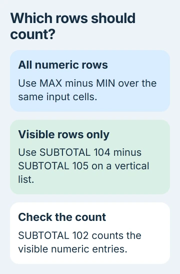
The SUBTOTAL reference lists those function numbers. SUBTOTAL handles filters in vertical lists; hiding a column in a horizontal selection doesn't work like hiding a row.

To count the visible numbers, use =SUBTOTAL(102,A2:A100). If the filter leaves no numbers, label the result as empty. Reporting zero without that explanation makes it look as though you measured a group with no spread.

Use the full-list formula when your report needs every measurement. Use the visible-list formula when the filter selects the group you want to measure. Choose based on the report's purpose, rather than the result you prefer.

Check what the range leaves out

Negative measurements work with the same subtraction. For practice values -4, -1, 2 and 7, the range is 11. Subtracting a negative minimum increases the difference; don't turn the inputs positive first.

The range depends only on the two extremes. Two groups can have the same range even when their middle values are very different. To describe the spread in more detail, calculate variance or standard deviation as your report requires.

If the answer still looks wrong, check the selected cells, COUNT result and separate maximum and minimum. If you need help from the workbook owner or support, share your exact formula and a few made-up numbers.

The Short Version

Subtract MIN from MAX over the same numeric cells. Keep summaries outside the inputs, distinguish blanks from zeros and check COUNT. For visible rows in a filtered column, subtract SUBTOTAL 105 from SUBTOTAL 104 instead.

Checked November 5, 2026.