Freeze the Top Row and First Column in Excel Together

You freeze the top row in Excel, then freeze the first column, and the row starts moving again. It's a frustrating loop when you just want the headings to stay with your data.

These commands don't build on each other. I'll show you the selection that keeps both in view, using desktop Excel for Windows, and how to reset it when too much of the sheet stays still.

Start at B2, then use Freeze Panes

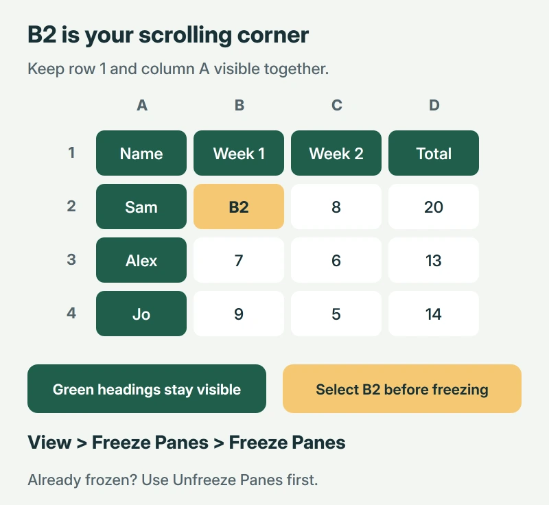
For row 1 and column A, select B2. Microsoft states that Freeze Panes keeps the rows preceding the selected cell and the columns to its left visible while you scroll.

B2 sits just after both headings. You're choosing where the scrolling part begins. You aren't selecting the headings themselves or changing anything inside their cells.

Status: Windows desktop Excel instructions checked against Microsoft's current Freeze Panes guide, 17 October 2026. Owner follow-ups were read; no workbook was tested here.

Use this sequence in your worksheet:

• If an area is already frozen, choose View > Freeze Panes > Unfreeze Panes first.
• Click B2, in column B, row 2.
• Choose View > Freeze Panes > Freeze Panes, using the general command in that menu.
• Scroll downward and then right to check that row 1 and column A remain visible.

Microsoft documents this Freeze Panes route. Don't follow it with Freeze Top Row or Freeze First Column; either separate choice changes what you just set.

Why half the sheet sometimes stays still

The selected cell decides the boundary. If you choose a cell far into the sheet, Excel keeps more rows and columns in place than you intended.

That happened in the Microsoft Q&A discussion about freezing both headings. The asker initially reported columns A through I and fourteen rows staying fixed.

A later reply confirmed success after understanding what the command meant by the current selection. Other owners report that the method worked too. You don't need a script for this.

I would check your selected cell next. If it isn't B2, use the reset sequence in the first section. You don't need to move the data around to change this boundary.

Choose a different corner for larger headings

Perhaps your worksheet has two heading rows, or names and account numbers in separate columns. The same selection rule handles both together. Count what must remain visible, then choose the first cell after that area.

Keep these visible	Select this cell
Row 1 and column A	B2
Rows 1 and 2, plus column A	B3
Row 1, plus columns A and B	C2
Rows 1 to 4, plus columns A to C	D5

These examples start at the worksheet's top and left edges. Freeze Panes doesn't pin a floating block in the middle while letting the cells around it scroll independently.

I would keep that area small. A large frozen section leaves less room for the part you're trying to read, especially on a small laptop screen.

If finding the corner is slow, our Excel keyboard routine explains jumping straight to a cell reference. That helps when the worksheet is much larger than the visible area.

When scrolling still feels wrong

Frozen panes can resemble a keyboard problem. If pressing an arrow moves the view instead of the selected cell, check Excel's Scroll Lock and selection modes.

The forum also includes an unresolved question from someone using Excel on a Mac. That owner reported a different menu, and the saved thread does not resolve their question.

The Short Version

Choose B2 and the general Freeze Panes command to keep row 1 and column A visible together. Clear an existing freeze first. For more heading rows or columns, choose the corner after the area you want to retain.

Where to Next

How many heading rows and columns does your sheet need to keep in view? Tell me the cell you selected if Excel holds the wrong area still, and whether you already had a freeze applied.