
Missing Excel data points usually come from a chart range that stops too soon, hidden source rows, or a series that's been filtered out. Start with Chart Design > Select Data and check whether the chart includes the missing cells.
A visible line without dots is a different problem: its markers may be turned off. A gap between two measurements can also be intentional when a source cell is empty. Match the symptom before changing your numbers.
In this guide
1. Include the missing rows in the chart range
Click the chart, open Chart Design, and choose Select Data. On desktop Excel, right-clicking the chart and choosing Select Data reaches the same window. Check the selected range against the rows on your worksheet.
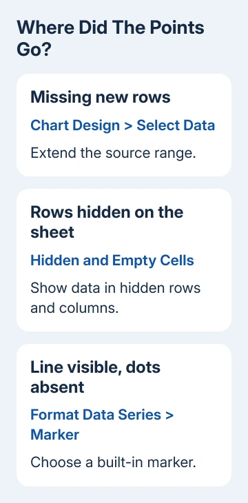
A chart made from rows 2 through 12 won't necessarily include measurements added in rows 13 through 20. Extend its source range to include the new rows, accept the change, and check the final date or category on the chart.
Under Legend Entries (Series), select the affected series and choose Edit. Confirm that its values refer to the cells holding the measurements. A series name can look right while its values still point to an older column.
For an XY scatter chart, check both Series X values and Series Y values. Each measurement needs its intended coordinate pair. Keep the two ranges lined up so the second x-value belongs to the second y-value.
The scatter plot setup explains how to arrange those paired columns. Use it when the dots appear at the wrong coordinates rather than disappearing completely.
Excel on Mac offers Chart Design > Select Data too, with different series controls. Choose the affected series there and check which cells it uses. The Windows buttons beside a chart may not be available.
If the last measurement now appears, the range was the problem. When the source already includes it, leave the range alone and check whether Excel is hiding that part of the series.
2. Restore a series hidden by the chart filter
In Excel for Windows, select the chart and look for the Chart Filters button beside it. Open Values, select the missing series or category, and choose Apply. Check whether the point returns without changing the worksheet.
Microsoft says chart filtering and removal work differently. A cleared filter checkbox hides the series; Remove deletes it from that chart.
If the filter doesn't list the series, check Select Data > Legend Entries (Series). To restore a deleted series, choose Add, then enter its name and source values. Filters can't restore a series removed from the chart.
Don't add a second copy if the original series is already present. Two identical series can sit on top of each other, making later formatting and legend changes confusing.
The filter button isn't offered in every Excel environment. On a Mac, use the series list in Select Data to inspect what the chart contains. Use desktop Excel for a setting unavailable in your browser edition.
If the series is present and selected but some rows remain absent, check the worksheet's hidden data settings next.
3. Let the chart include hidden worksheet data
Hiding worksheet rows or columns normally hides their chart data too. This is separate from a chart's own filter. Think back to whether the points vanished after you hid a section of the sheet.
Select the chart, choose Chart Design > Select Data, then open Hidden and Empty Cells. Select Show data in hidden rows and columns and confirm the dialogs. Check the chart while those source rows are still hidden.
That option lets you keep rows hidden on the worksheet while showing their measurements on the chart. Unhide the rows to confirm their connection to the missing points, then hide them again if this chart setting works.
A filtered table needs extra care: filtering rows isn't the same as hiding them manually. Clear the worksheet filter temporarily and see whether the missing measurements return before treating this checkbox as the answer.
If they return with the worksheet filter cleared, decide which records the chart should represent. Showing excluded records would change the meaning of a chart meant to follow that filter.
When all source rows are available and a gap remains, inspect the cell at that position rather than changing visibility again.
4. Choose how to display a real gap
Click the cell for the missing measurement and read the formula bar. An empty cell, an error such as #N/A, and a real zero mean different things. Never substitute zero for a missing measurement simply to fill a gap.
In Hidden and Empty Cells, the Show empty cells as choices include Gaps, Zero, and, for supported chart types, Connect data points with line. Choose the behavior that matches your data.
Gaps leaves the absence visible. Zero plots an empty cell at zero. Connect data points with line joins surrounding measurements without creating a measured value for the missing position.
A scatter chart showing markers without connecting lines can't use the connecting-line option. Its empty-cell choices are gaps or zero. That limitation doesn't mean the workbook is damaged.
Some Microsoft 365 Insider builds offer Show #N/A as an empty cell. If you don't see that checkbox, use the controls your version offers instead of changing formulas to match another screen.
A cell containing a formula that returns an empty string isn't the same as a truly empty cell. Check the formula before assuming the empty-cell setting explains its behavior. If the formula is wrong, correct it in the worksheet.
If the worksheet displays formula text instead of a result, use the formula display checks. A chart needs usable values, so fix the cells before changing the chart.
5. Make plotted points visible with markers
A line that reaches every category but has no dots can have its markers disabled. Select the series, open Format Data Series, and find Marker under its formatting options. Choose a built-in marker and a readable size.
Use a fill that stands out from the plot area. If several series share the same coordinates, one can cover another. Use the chart's formatting selection control to select each series to see which series you're changing.
I'd check markers before rebuilding a chart whose line already follows the expected values. Rebuilding won't help if the replacement uses another line-only style.
If a small test chart from the same cells works but the original still fails, save a separate workbook copy and ask Excel Support to inspect that chart. Include your Excel version, chart type, source ranges, and which point should appear.
The Short Version
Check the source range first, then chart filters and hidden rows. Treat blank cells separately from zeros, and enable markers when the line is visible but its dots aren't. Correct the source data before rebuilding the chart.
Checked November 13, 2026.