

Excel uses <> for not equal. Enter =A2<>B2 to check whether two cells differ: TRUE means they don't match, and FALSE means they do. Start with that direct comparison before putting it inside an IF or counting formula.
The same comparison works in Excel for Windows, Mac, and the web. Choose the formula based on what you want back: a true-or-false result, a label for each row, or a count or total for rows that don't match a condition.
In this guide
Compare two cells and check the result
Put your first value in A2 and the second in B2. Select an empty result cell, type =A2<>B2, and press Enter. Use the less-than sign followed immediately by the greater-than sign, with no space between them.
For a simple check, enter 14 in A2 and 19 in B2. The result is TRUE. Change B2 to 14 and the result becomes FALSE. Try this small example so you know what the results mean before comparing a long sheet.
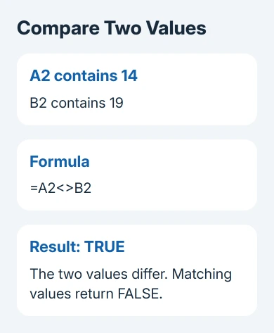
Microsoft's calculation-operator reference lists <> as the not-equal operator. The mathematical not-equal character and the programming-style != aren't replacements for it in an ordinary Excel formula.
Cell references don't need quotation marks. Comparing A2 with B2 means reading the contents of those cells. Putting a reference inside quotes would turn it into text instead of reading that cell's value.
If the formula itself stays visible instead of a result, check how the formula was entered and whether Excel is calculating it. The Excel calculation checks cover text-formatted cells, visible formulas, and results that aren't updating.
Compare a value with text or a fixed cell
To check that a status isn't Closed, use this formula:
=A2<>"Closed"The text needs straight double quotes; a cell reference doesn't. This returns TRUE for other status text and FALSE when A2 contains Closed. Type the status exactly as your sheet uses it, including any intentional spaces.
For a numeric comparison, use a number without text quotes, such as =A2<>14. A number stored as text can behave differently from a number Excel recognizes, so check the stored data when apparently identical values don't match.
When the comparison target is in one fixed cell, use dollar signs to hold its address. For example, =A2<>$E$1 compares each row against the value in E1 as you copy that formula through later rows.
Without those dollar signs, copying the formula down changes E1 to E2, E3, and so on. That can make later rows appear wrong even though the comparison operator is correctly comparing the cells named in the formula.
Test the first copied row by selecting its result and reading the formula bar. Check that the input reference changed to the next row and the comparison cell stayed at E1. Then fill the remaining rows.
Return a useful label with IF
A TRUE or FALSE result is enough for a check column. Use IF when the result should say something useful to the person reviewing the sheet. Put the not-equal test first inside IF:
=IF(A2<>B2,"Review","Match")With 14 in A2 and 19 in B2, this displays Review. When both contain 14, it displays Match. IF uses the first label when the test is TRUE and the second when it's FALSE.
Choose labels that explain the action rather than implying a mismatch is automatically an error. Two order amounts can differ for a valid reason; Review asks someone to check without changing the original data.
If your worksheet separates function inputs with semicolons, use those instead of commas. Keep <> unchanged. Those separators depend on regional settings, rather than whether the workbook is open on Windows or Mac.
To reverse a larger logical test, use the Excel NOT function. A direct <> comparison is easier to read when all you need is whether these two values differ.
Count or add rows that exclude a condition
Use COUNTIF to count entries whose status isn't Closed. COUNTIF needs the condition as text, so put the operator and status together inside quotes:
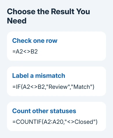
=COUNTIF(A2:A20,"<>Closed")This counts entries in A2 through A20 that meet the not-Closed condition. Check it against a small sample containing known statuses before using the result in a report. Don't assume every row in a real sheet has a completed status.
If the excluded value is stored in E1, join the quoted operator to the cell reference:
=COUNTIF(A2:A20,"<>"&E1)The ampersand joins the operator text with the value in E1. Writing E1 inside the same quoted text would ask Excel about those characters rather than the value in that cell.
For a total instead of a count, SUMIF uses the same kind of condition. If column A holds status and column B holds amounts, this adds the amounts whose status isn't Closed:
=SUMIF(A2:A20,"<>Closed",B2:B20)Keep status and amount ranges on the same rows. If the amount range starts on the wrong row, the total can look reasonable while adding the wrong records. Test with a few amounts you can add yourself before extending the ranges.
Handle blanks and letter case intentionally
To check whether a cell isn't empty for a simple formula test, compare it with an empty text string:
=A2<>""An empty string has nothing between its two quotes. A space inside the quotes is a different value. This matters when a cell looks blank but actually contains spaces, or when another formula returns empty text.
Ordinary text comparisons don't distinguish capitalization. If letter case must matter, use EXACT for the comparison and reverse that result with NOT:
=NOT(EXACT(A2,B2))This can flag a difference between the same letters with different capitalization. Use it for codes or IDs where capitalization matters, rather than treating capitalization as a mismatch in every name or status list.
If a result still looks wrong, open each input's formula bar and check for stray spaces, formulas, and stored values. Two cells can look the same on screen while storing different numbers or text.
For help with a stubborn workbook, give Microsoft Excel Support the formula and two sample inputs with private details removed. Include the result you expected and whether case, blanks, or numbers stored as text should count as different.
The Short Version
Use =A2<>B2 for a direct comparison, IF to return labels, and quoted <> criteria with COUNTIF or SUMIF. Keep fixed references when copying, and decide how blanks and capitalization should behave before trusting a column of results.
Checked November 13, 2026.