

Excel's NOT function turns a TRUE result into FALSE, and FALSE into TRUE. Put the condition inside =NOT(...); for example, =NOT(A2>100) returns TRUE when A2 isn't greater than 100.
Use it when reversing a condition makes your formula easier to read. It works with IF, AND and OR, but the placement of the parentheses changes which result you reverse. Start with a single test before combining conditions.
In this guide
Start with one condition you can check by hand
In a blank part of your sheet, enter 120 in A2. In B2, enter =A2>100. Excel displays TRUE, because 120 is greater than 100. Now enter =NOT(A2>100) in C2.
C2 displays FALSE. NOT reverses the TRUE or FALSE answer from the comparison; it doesn't change the value stored in A2. This makes it useful for a separate results column alongside your original records.
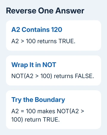
Change A2 to 80. B2 becomes FALSE and C2 becomes TRUE. Finally, try 100. The original greater-than test is FALSE at the boundary, so the NOT version returns TRUE there too.
That last check matters. Not greater than 100 includes 100 itself. It means the same as A2<=100 for the numeric values in this example, rather than the stricter A2<100.
Microsoft's NOT function reference lists one required input, called an argument: a value or expression Excel can read as TRUE or FALSE. The expression can contain other functions.
Give IF the reversed result and choose the output
Suppose column A contains amounts and you want a label for amounts that don't exceed 100. In B2, enter this formula, then press Enter:
=IF(NOT(A2>100),"Within limit","Over limit")With 80 or 100 in A2, the result is Within limit. With 120, it's Over limit. IF uses its first output when the condition is TRUE and its second output when the condition is FALSE.
The closing parenthesis after 100 finishes NOT before IF's two output choices begin. Text labels go inside straight double quotes. Cell references, numeric limits and function names don't need those quotes.
If your Excel uses semicolons between arguments, replace the separating commas with semicolons. Leave the rest of the formula and its parentheses as they are. Local settings can change the separator without changing the test.
I'd use the simpler comparison A2<=100 here in a working sheet. NOT earns its place when you already have a longer condition to reverse, rather than as extra punctuation around every comparison.
For two cells that should differ, write a direct not-equal comparison and use IF only when the result needs a label.
Reverse a combined condition at the right level
For a range check, enter 10 in A2 and 20 in B2. The formula =AND(A2>=0,B2>=0) returns TRUE because both values are zero or positive. AND needs every condition to be TRUE.
To flag any row where that combined check fails, use:
=NOT(AND(A2>=0,B2>=0))With 10 and 20, it returns FALSE. Change A2 to -1 and leave B2 at 20: it returns TRUE. If either number is negative, AND returns FALSE, and NOT reverses that combined result.
Moving NOT inside AND gives a different rule. =AND(NOT(A2>=0),NOT(B2>=0)) returns TRUE only when both numbers are negative. It doesn't flag the row containing -1 and 20.
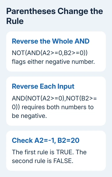
Read the formula from the innermost parentheses outward. Work out the comparisons first, then AND or OR, then any surrounding NOT. That order helps you see which answer changes before IF chooses a label.
Use NOT with OR when neither condition should apply
OR returns TRUE when at least one of its conditions is TRUE. To check whether either number is negative, use =OR(A2<0,B2<0). It returns TRUE for -1 and 20, or for 10 and -1.
Wrap that whole expression in NOT to require that neither number is negative:
=NOT(OR(A2<0,B2<0))With 10 and 20, the result is TRUE. With either negative value, it's FALSE. For these numeric examples, this gives the same result as =AND(A2>=0,B2>=0).
Choose the wording that matches your rule. A sheet described as rejecting negative inputs might read naturally with NOT around OR. If your rule is that both numbers must be zero or positive, AND may be clearer.
While building a longer formula, put each test in a temporary helper column so you can see its result. That lets you check the combined condition before adding labels or calculations to the final result.
Check real inputs before filling the formula down
Test the boundary and both sides of it using the kind of data your sheet contains. For an amount limit, check the exact limit too. For a rule with two inputs, also try cases where just one input fails.
Use a small example with known expected answers before copying the formula through your records. Excel can accept a formula that still applies the wrong rule, especially when NOT reverses the wrong part of it.
Blank inputs need their own decision. An empty cell and a formula displaying empty text don't always behave the same way. The IF not blank examples explain which check fits those two situations.
Don't assume NOT cleans imported data or turns an error into a usable answer. If a referenced calculation already has an error, fix that input or function rather than relying on a reversed condition to hide it.
When copying a formula, check whether its cell references should move with each row. A limit stored in one fixed cell needs an absolute reference such as $D$1; the record being tested normally keeps a changing row reference.
When Excel won't accept the formula
Check the function spelling, parentheses and argument separator in the formula bar. NOT takes one argument, so two separate conditions need to be combined with a function such as AND or OR before NOT reverses them.
For #NAME?, use the unrecognized-name checks to correct the part Excel can't read. In a localized Excel installation, use its function suggestions if the English name isn't recognized.
If a short example works but the real formula doesn't, give the workbook author the formula, sample inputs and expected result. Replace private records with made-up values that reproduce the same answer before asking for help.
The Short Version
Put one logical test inside NOT to reverse its answer. NOT around an entire AND or OR expression reverses the combined result. Check boundary values and single-failure cases before copying the formula across your data.
Checked November 12, 2026.