

Excel can lose the parentheses choice for negative numbers because of Windows regional settings. Change the negative-number pattern in Region, or apply a custom number format when only this workbook needs brackets.
When the choice is there but a cell ignores it, check whether the amount is stored as text. That problem needs conversion before a number format can affect it.
In this guide
1. Choose the negative-number style in Format Cells
Select a cell containing a negative amount. In Excel for Windows, press Ctrl+1. On a Mac, press Command+1. Choose Number or Currency in the category list and inspect the negative-number choices.
Choose an example with parentheses, then select OK. A numeric value such as -125 should display with parentheses in the chosen format, while the value used in calculations stays negative.
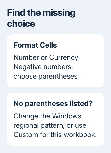
If the parentheses option is missing, continue to the Windows regional setting or the workbook-only custom code. Clicking the same minus-sign choice again won't add a pattern that isn't in the list.
If the option exists but the cell doesn't change, go to the text check. A format changes how a number looks; it doesn't automatically turn every pasted text string into a number.
Keep the distinction between a negative value and its display. Don't type parentheses into hundreds of cells just to change the report's appearance. That can leave a mixture of text entries and real numbers.
2. Restore missing choices in Windows Region
Microsoft's missing-parentheses fix uses the regional number and currency patterns. Close Excel before changing them so it picks up the new settings when you reopen it.
Open Start, search for Control Panel, and launch it. In Category view, open Clock and Region > Region, or choose Change date, time, or number formats. In icon view, open Region directly.
On Formats, choose Additional settings. Under Numbers, set Negative number format to the example with parentheses, shown as (1.1). Under Currency, set Negative currency format to ($1.1).
Select OK in both dialogs, then reopen Excel. In Format Cells, apply the Number or Currency pattern your report needs. Check both an ordinary amount and a currency amount if your report uses both.
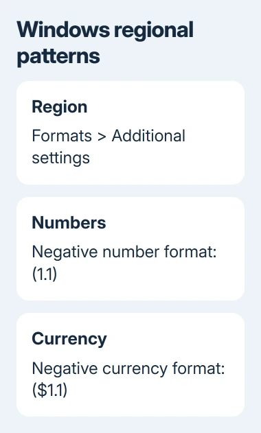
This changes the computer's regional formatting for other applications too. Note the previous patterns first so you can restore them if they conflict with your workplace's formatting rules.
Windows 10 and 11 both retain these Control Panel regional controls. You can choose a negative-number pattern without changing the Windows display language or the region itself.
One owner restored the bracket choices through Additional settings while retaining English (Canada). Another fixed it by changing the region, but that broader change isn't needed.
On a managed computer, ask IT to change the regional pattern if you can't edit those settings. For one report, use the custom-format method instead of changing a company-wide preference.
3. Use a custom code for this workbook
I'd choose a workbook-specific code if the computer's other number displays already suit you. It changes selected cells without requiring a new Windows regional preference.
Select the amounts and open Format Cells again. Under Number, choose Custom. In Type, enter this two-section code, then select OK:
#,##0.00;(#,##0.00)The first section displays positive numbers and zero. The second, after the semicolon, displays negative numbers inside parentheses. For an English US number display, -1234.5 becomes (1,234.50).
The code belongs in Type, not in the worksheet cell or formula bar. Typing it into a cell creates text instead of formatting the amount that's already there.
For whole-number reports, use #,##0;(#,##0) instead. Keep two decimal placeholders for prices that need cents. A whole-number display can hide fractional amounts without removing them from calculations.
In Excel for Mac, Home > Number Format > More Number Formats also opens the dialog. Choose Custom, edit Type, and save the workbook. Custom formats are stored with that workbook, rather than becoming a new global default.
Regional decimal and thousands separators can change the code Excel expects. Start with a local built-in number pattern and add a second section with parentheses if the example doesn't match your locale.
The Excel hidden-value guide explains another use of custom format sections. For this repair, both positive and negative amounts should remain visible; don't use a code that hides them.
4. Convert amounts that are really text
Read the formula bar for an amount that still resists formatting. Imported amounts can contain a leading apostrophe, spaces or a currency symbol stored as part of the text. Choosing Number doesn't necessarily remove those characters.
In a spare cell, enter =ISNUMBER(A2), replacing A2 with the affected cell. TRUE means Excel recognizes a number. FALSE means changing its numeric display alone won't solve this case.
When Excel flags text amounts with an error indicator, select those cells and choose Convert to Number from the warning menu. Reapply your format with parentheses after conversion.
For an amount stored as plain text, =VALUE(A2) can convert recognized text in a helper column. Check the result before replacing the original. Its decimal and thousands separators must match the regional settings used for conversion.
A formula using TEXT returns text even when the result looks numeric. Format the underlying number when calculations must keep using it, rather than trying to change the output string with Format Cells.
If the issue affects formulas too, the Excel formula-display checks help distinguish text entries from a formula that's being displayed instead of calculated.
When the display still isn't right
Check for a conditional rule that applies its own number format under Home > Conditional Formatting > Manage Rules. A rule can control what the cell shows when its condition matches, even after its ordinary format changes.
If a fresh numeric entry in a blank workbook also fails, send your Office administrator the Excel version, regional patterns and the format code. Ask them to review Office installation and policies before changing your original amounts.
On a Mac, try the workbook's custom code first when only the parentheses choice is missing. If built-in options remain wrong, install available macOS updates and ask support to review the Mac's regional settings.
The Short Version
Restore missing parentheses through Windows Region, or use a two-section custom format for selected cells. Convert text amounts before formatting them. The value stays negative in calculations when its minus sign becomes parentheses.
Checked November 16, 2026.