

VLOOKUP's approximate match doesn't find the nearest number in both directions. It can return 9 for 9.9 even when 10 is available. Use INDEX and MATCH with MIN and ABS to compare distances and return the nearest row's value.
The same formula can return the number itself or the label beside it. Choose the column with the result you want, then enter the formula using the shortcut your Excel version needs.
In this guide
1. Replace the approximate lookup with a distance comparison
Put the numbers you're choosing between in A1:A2, their labels in B1:B2, and the number you're looking up in C1. For a small example, use 9 and 10 in column A, with X and Y beside them, and 9.9 in C1.
Enter this in an empty result cell:
=INDEX(B1:B2,MATCH(MIN(ABS(A1:A2-C1)),ABS(A1:A2-C1),0))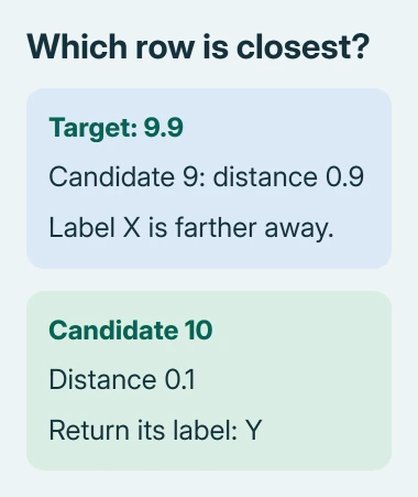
The result should be Y, because 10 is only 0.1 away from 9.9. The other candidate, 9, is 0.9 away. A result of Y shows that the formula found the nearest number and returned the label beside it.
In Excel for Microsoft 365, press Enter. In Excel 2010 and other editions using legacy array entry, hold Ctrl + Shift while pressing Enter. An array formula calculates across several values together.
Excel adds curly braces around a correctly entered legacy array formula. Don't type those braces yourself. If you later edit the formula in a legacy version, confirm it again with Ctrl + Shift + Enter.
Microsoft's array formula instructions explain the difference between current Microsoft 365 entry and older array formulas. If the formula produces an error, check entry and ranges before changing the lookup logic.
2. Return the label or the nearest number
The first range after INDEX tells Excel which column to return a value from. In the example, B1:B2 returns X or Y. To return 9 or 10 instead, change only that first range:
=INDEX(A1:A2,MATCH(MIN(ABS(A1:A2-C1)),ABS(A1:A2-C1),0))Keep the two ranges inside ABS pointing at the numbers you're comparing. Those are the values Excel compares with C1. Replacing them with the label column would ask Excel to subtract a number from text.
An owner in Microsoft's discussion confirmed the nearest-number calculation worked, then explained that they needed the corresponding text. The label version solves that second part by returning column B from the same matched row.
A second VLOOKUP isn't needed to retrieve that row's label. INDEX already has the row position it needs. Adding a second lookup makes the formula harder to follow and can introduce a separate matching problem.
If you get a number that looks reasonable but expected a product, name or code, check the first INDEX range. If the result is an error instead, move to the range and data checks in section 5.
3. Lock the table before filling the formula down
For a larger table, suppose your numbers are in A1:A20, their labels are in B1:B20, and lookup values begin in C1. Put this in D1:
=INDEX($B$1:$B$20,MATCH(MIN(ABS($A$1:$A$20-C1)),ABS($A$1:$A$20-C1),0))Use the Enter shortcut for your version of Excel, then fill the result cell down beside your lookup values. Dollar signs prevent the table references from moving. C1 changes to C2, C3 and so on for each new row.
Check the first few results manually before filling hundreds of rows. For each lookup value, compare the nearest candidates on either side. This catches a shifted range or a wrong return column while the example is still easy to read.
If the first result works and later results don't, select one of the later formulas and inspect its references. Both candidate ranges and the return range should still cover the same original rows.
I'd keep the test table small until the result column is right. A two-row example makes a mistaken reference much easier to see than a full worksheet of frequencies or prices.
4. Understand why the result changes
ABS removes the minus sign from each difference. That makes a candidate 0.1 less than your target just as close as one 0.1 greater. MIN chooses the smallest of those distances.
MATCH finds that distance's position. Its final 0 asks for an exact match to the distance, rather than another approximate lookup. INDEX uses the position to retrieve the corresponding entry from your chosen return range.
For this formula, the candidate numbers don't need sorting. You're comparing every candidate's distance rather than searching for the next smaller entry in an ordered list.
An exact candidate has a distance of zero and wins. If two distances are exactly equal, MATCH returns the first matching position. The formula returns one result, so it won't list every tied candidate or every duplicate label.
Decimals that display equally can have different stored values. A later reply shows that issue with 5.0, 5.2 and a target of 5.1. Decide your required precision before adding rounding to a business calculation.
5. Fix entry, range and data problems
Keep the number and result ranges the same length, with each number and its label on the same row. If column A starts at row 2 but INDEX starts at row 1, you'll get a label from the wrong row even when the distance calculation is correct.
Use only the populated numeric rows while checking the formula. Blank cells, text, headings and existing errors don't belong in the candidate range. Don't expand A1:A20 to an entire column simply to avoid checking the last data row.
If your Excel installation uses semicolons between arguments, replace the formula's argument commas with semicolons. Keep the decimal separator your installation expects when entering the lookup number.
A cell showing the formula as text needs the separate formula display checks. A standard exact lookup returning #N/A calls for the VLOOKUP error checks instead.
If a small clean example works but your real table doesn't, share a few rows with private details removed, the lookup value, the formula and the expected answer with your spreadsheet support team. Include how ties should be handled.
The Short Version
Compare distances with MIN and ABS, use MATCH to locate the nearest row, and let INDEX return its number or label. Lock the reference table before filling down. Legacy Excel needs Ctrl + Shift + Enter; current Microsoft 365 uses Enter.
Checked November 17, 2026.