
An MMULT #VALUE! error often means a selected cell contains text or is empty, or the ranges have mismatched row and column counts. Check both ranges first. If it works at 5×5 but fails at 6×6, one of the added cells may be the problem.
Excel 2016 can multiply two 10×10 matrices. The important size rule is that the first matrix's column count must equal the second matrix's row count. Older Excel also needs the result entered as an array formula.
In this guide
1. Match the two ranges before changing the formula
Click the formula and read its two references in the formula bar. For example, =MMULT(A1:J10,L1:U10) multiplies two ten-row, ten-column blocks. Both references must stop before any headings or totals.
Matrix multiplication combines rows from the first block with columns from the second. It differs from multiplying matching cells individually. If matching-cell multiplication is the task, MMULT is the wrong function.
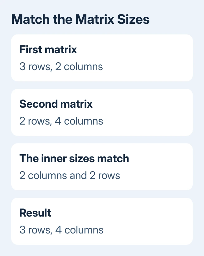
Use =COLUMNS(A1:J10) and =ROWS(L1:U10) in spare cells to compare the first range's columns with the second range's rows. They should return the same number. This is more reliable than counting a wide selection by eye.
The result takes the first block's row count and the second block's column count. A 3×2 first matrix multiplied by a 2×4 second matrix produces 3×4 results. The inputs don't have to be square or the same shape.
If those counts differ, correct the mistaken reference. Don't trim a required row just to silence the error. When the references fit, check whether every selected input is actually a number.
2. Count numeric cells in each matrix
In spare cells outside both matrices, enter =COUNT(A1:J10) and =COUNT(L1:U10). Each ten-by-ten input should contain 100 numeric cells. A smaller count means at least one cell isn't being counted as a number.
Then compare each count with =ROWS(A1:J10)*COLUMNS(A1:J10), adapting the reference for the second matrix. This calculates the number of selected positions, so the check still works for a rectangular block.
MMULT needs a number in every selected cell, including any missing measurements. A formula returning empty text also needs attention even though the grid looks empty. Check the formula bar when the sheet doesn't explain the short count.
Click a suspect input and use a spare formula such as =ISNUMBER(A6) to see whether it is numeric. FALSE tells you to review that cell's contents. It doesn't tell you which replacement value belongs in your data.
Correct an accidental label or numeric text at its source. If a missing entry truly means zero in this calculation, enter a numeric 0 there. An unknown measurement shouldn't become zero simply to get an answer.
For broader input cleanup, the Excel #VALUE! checks explain stored text and spaces. For MMULT, every cell in both matrices needs to contain a valid number.
3. Inspect the added rows when only larger blocks fail
When a 5×5 version works and a 6×6 version fails, compare exactly what the larger formula adds. That includes the new row and new column in both input matrices. Checking only the first block can miss the offending cell.
Microsoft's MMULT requirements list empty or text inputs and incompatible dimensions as causes of #VALUE!. There isn't a five-by-five restriction in those requirements.
One owner fixed the apparent size limit by correcting a mistaken percentage entry. Their explanation mixed up decimals and percentages, so don't take it as a reason to replace every percentage in your workbook.
A real numeric percentage is still a number. 9.2% represents 0.092, while 9.2 is a much larger value. Choose the amount your calculation needs; a successful formula with the wrong amounts is still the wrong answer.
Review the added cells in the formula bar and source records. Check imported numbers carefully if their decimal separators don't match your settings. Changing only a cell's visible format doesn't convert text into a number.
If the count is correct but the error remains, inspect inputs containing formulas. Fix any calculation error at its source. Keep the error visible while tracing it instead of wrapping the result in IFERROR.
4. Enter the result for the Excel version you use
In current Microsoft 365, select the top-left destination cell, type the MMULT formula, and press Enter. Excel fills neighboring cells with the other results automatically, a behavior called spilling. Leave the required result area clear.
In Excel 2016, select the whole output block first. For two 10×10 inputs, that's a separate ten-row, ten-column destination. Type the formula with the selection still active, then press Ctrl+Shift+Enter together on Windows.
Excel supplies the array formula's curly brackets. Don't type those brackets into the formula yourself. The selected output block should show the matrix results rather than a single value at its top-left corner.
Legacy Mac Excel uses Control+Shift+Return for array entry. Current Microsoft 365 Mac uses normal Return for a dynamic array. Use the method for your version rather than repeatedly trying Windows shortcuts.
In older Excel, entering the formula without the array shortcut can return only one result. That's a separate issue from bad input ranges. Once the formula calculates, check the whole output block for every result you need.
If Excel shows #SPILL! instead, an occupied output area needs attention. The Excel spill-error checks cover blocked dynamic-array results. Don't overwrite useful cells to make space without checking them first.
5. Give a remaining failure a small reproducible example
I'd check the inputs and entry method before repairing Office. They check what MMULT needs to work and leave the rest of your workbook intact.
If it still fails, create two small numeric matrices in a new workbook. Record their references, formula, Excel version and entry method. That gives the workbook's author a way to compare your data with a fresh Excel calculation.
Send that example to the spreadsheet's author or Microsoft support through Help. Ask them to check MMULT's input types, dimensions and array-entry method. Replace private measurements with harmless sample numbers before sharing the file.
The Short Version
The first matrix needs as many columns as the second has rows, and both need numeric inputs. Inspect cells added by a larger range. Use Enter in current Microsoft 365 and array entry with the whole output selected in Excel 2016.
Checked November 17, 2026.