

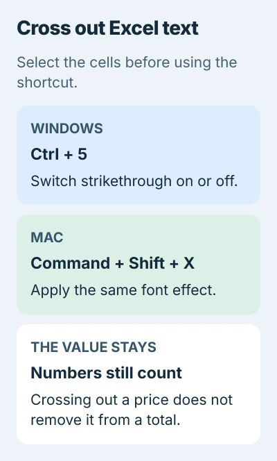
Select a cell and press Ctrl+5 to cross out its contents in Excel for Windows. On a Mac, use Command+Shift+X. The effect is called strikethrough, and it changes how the text looks while keeping the original value.
For just a few words inside a cell, select those words while editing the cell first. Otherwise, the shortcut applies to the entire selection.
Cross out the selected cells with a shortcut
Click the cell containing the item you want to mark complete. Finish any typing by pressing Enter, then select that cell again. Hold Ctrl and press 5 once on Windows, or hold Command and Shift while pressing X on Mac.
Microsoft lists both commands in its Excel keyboard shortcuts. Each command switches strikethrough on or off, so the same shortcut can remove it later.
For several neighboring cells, drag across the cells you need before using the shortcut. To cross out a task description without changing its date or price, select just the description cells instead of entire rows.
Check a cell that contains ordinary text. You should see a line through the middle of its letters and the same content in the formula bar.
A crossed-out number still takes part in calculations. For example, marking a price as canceled doesn't remove that price from a total. Use a separate status column or change the calculation when the number should stop counting.
If the shortcut changes something outside Excel, click back into the worksheet and try the menu method next. Your browser or another app may be using that shortcut before Excel gets it.
Find Strikethrough in the Font settings
With the cells selected in Windows, Ctrl+1 opens Format Cells. Choose Font, select Strikethrough under Effects, and confirm with OK. The formatting appears when the dialog closes.
On the Home tab, the Font group's small launcher button opens these text-formatting controls. Use it if a keyboard utility has taken over the shortcut.
On Mac, open Format > Cells, then choose the Font tab and its Strikethrough option. Command+1 also opens Format Cells. Keep your cells selected while opening the dialog so Excel formats the right ones.
When only some selected cells have strikethrough, the check box can show a mixed setting. Select Strikethrough to give them all the same setting, then check a few cells at both ends of the range.
In a browser workbook, select your cells and choose Home > Font Settings. Select Strikethrough in the Format Cells dialog and confirm. The font controls can be in a different place from desktop Excel.
I'd use the Font dialog for a mixed selection. It's easier to see the setting you're applying than to press the shortcut repeatedly while guessing which cells already had it.
Mark only certain words inside one cell
Double-click a cell containing ordinary text. Drag over the words you want to cross out, leaving the other characters unselected. Apply the Windows or Mac shortcut, then press Enter to finish editing.
For example, a task cell can contain an old appointment time followed by its replacement. Selecting only the old time lets you keep both pieces of information while showing which one no longer applies.
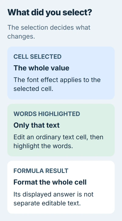
Use the formula bar to select text when editing inside the cell is awkward. Make sure the words you want to cross out are highlighted before using strikethrough.
For text you've typed into the cell, you can format individual words. That won't work with a formula's displayed result. Cross out the whole cell instead, or keep the description in a separate text cell.
If the wrong words changed, undo the action and select the text again. Your description stays intact, so you don't need to retype it or turn the cell into a picture.
For labels with raised characters, the Excel superscript guide covers that separate effect. Pick the format that makes your label clear.
Remove the effect without clearing your other formatting
Select the crossed-out cells, open Font settings, and clear Strikethrough. For a cell where only selected words have the effect, highlight those words in editing mode before removing it.
Leave Clear Formats alone when you're only removing strikethrough. It can also remove your number format, fill, font and other formatting from the selected cells.
If the stroke returns after a cell's value changes, inspect Home > Conditional Formatting > Manage Rules. A rule can apply formatting automatically when its condition is met, even after you change a cell's ordinary font settings.
Show the rules for the affected worksheet or selection and check which cells each one covers. In a shared workbook, ask its owner before changing a rule you don't understand.
For a list that should react to a completion status, use a conditional-formatting formula. It applies the effect automatically.
To hide a column without deleting it, use the Excel column-hiding controls. Crossing out its contents leaves them visible.
When Excel will not let you change the font
Check whether the workbook is open for viewing or the worksheet is protected. Ask for editing permission or ask its owner to unlock the sheet. Reinstalling Excel won't change those restrictions.
If strikethrough works in a blank workbook but fails in one shared file, tell its owner. If it also fails in a new file, give support your Excel version, whether you're using Windows, Mac or a browser, and the command you tried.
The Short Version
Use Ctrl+5 on Windows or Command+Shift+X on Mac. Select individual words in editing mode for partial text formatting, and clear only Strikethrough when removing it. Crossed-out values remain in your calculations.
Checked November 5, 2026.

Isaac Smith is the founder and editor of PC Glance, a website that covers computers, laptops, and technology. He is a tech enthusiast and a computer geek who loves to share his insights and help his readers make smart choices when buying tech gadgets or laptops. He is always curious and updated about the latest tech trends.