Fix the #REF! Error in Excel Without Hiding Bad Formulas

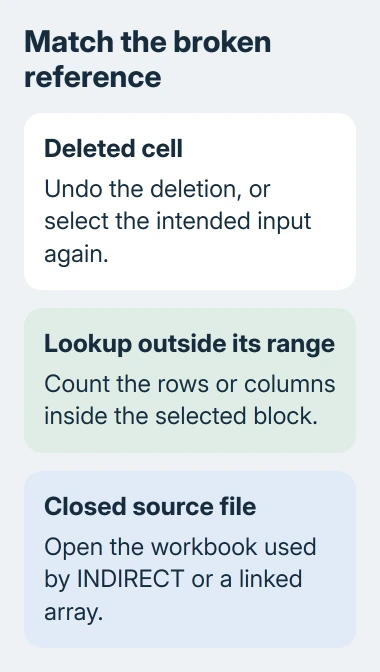
Excel's #REF! error often starts after a formula's input cells are deleted. Undo that change if it just happened. For VLOOKUP, INDEX or a linked workbook, check the requested range or open the source file instead.

Changing the cell's appearance won't repair the calculation. Click one affected cell and read its formula bar: #REF! inside the formula means an input needs restoring. If the formula looks intact, check its ranges.

1. Undo the deletion before rebuilding the formula

If the error appeared immediately after deleting or moving cells, reverse the change with Undo if Excel still offers it. On Windows press Ctrl+Z; on Mac press Command+Z. Check that the missing data and the calculated result return together.

I'd try Undo before editing a dozen formulas. One mistaken deletion can break many dependent cells, and undoing that action is easier to check than rebuilding each reference from memory.

If you've made useful changes since the mistake, save a separate copy before working backward. That gives you a place to recover those later edits without overwriting the only copy of the workbook.

Suppose a total adds three individual cells with =SUM(B2,C2,D2). Deleting column C can leave a broken reference inside that formula. Emptying a cell's contents is different from removing its column from the worksheet.

When removing records is the goal, delete the intended rows and inspect the totals afterward. Don't keep deleting neighboring cells to make the error disappear; the formula still needs to calculate what it did before.

2. Replace a broken reference with the intended cells

Click the first error and read the formula shown in the formula bar. If it contains #REF!, work out which input used to be there. A nearby working formula, a previous saved copy, or the workbook's owner can help you identify it.

Edit the formula and select the correct input cell or range. Press Enter, then compare the result with the source values. A number appearing is only the first check; it must be the number the formula was meant to calculate.

For a continuous total, a range such as =SUM(B2:D2) can handle deletion of a column within that range more cleanly than a list of separate references. Use it only when all cells in that range belong in the total.

Take care when subtotals or notes sit between the cells you're adding. Replacing every broken formula with a wider SUM can silently count something twice. Match the range to the calculation, then check a small example by hand.

If the selected formula looks correct, follow the cells it uses. One input may already contain #REF!, passing the error into a total that hasn't lost any references itself.

Repair the earliest broken calculation rather than each result that depends on it.

3. Count VLOOKUP's columns from the selected range

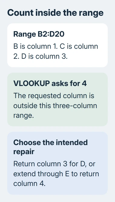
A VLOOKUP can return #REF! even when it contains no deleted-cell marker. Its return-column number must fit inside the lookup range. Count from that range's left edge, rather than from the worksheet's A column.

For example, =VLOOKUP(G2,B2:D20,4,FALSE) asks for a fourth column from a range that contains only three: B, C and D. There isn't a fourth column in that table.

If column D contains the answer, change the return-column number to 3. If column E contains the answer, extend the range through E and keep 4. Those are different repairs because they return different information.

Try a lookup value whose answer you already know. When the formula returns that expected value, fill the corrected formula into the other rows and check that the lookup range stays where you intended.

For a missing matching item, #N/A is a different problem. Changing a column number to repair #REF! won't create a record that isn't in the lookup table. Read the actual error before changing the formula again.

4. Keep INDEX's row and column inside its array

INDEX uses positions within its selected block. In =INDEX(B2:D8,8,2), the block contains seven rows, so asking for its eighth row returns #REF!. The worksheet's row numbers aren't the positions used here.

Count B2 as row 1 of this block and B8 as row 7. If the intended answer is in C8, the row position is 7 and the column position is 2: =INDEX(B2:D8,7,2).

If the intended source really extends through row 9, enlarge the array instead. Don't reduce the position just to clear the error. That can return a number from the wrong record.

When MATCH supplies the position inside a longer formula, inspect the range used by MATCH too. Its positions need to line up with the array given to INDEX. Compare the first and last records in both ranges.

These fixes work the same way in current desktop Excel on Windows and Mac. Commas in these examples separate function arguments; installations using a different regional list separator may show semicolons instead.

5. Open a source workbook used by INDIRECT or arrays

A formula using INDIRECT, which turns text into a cell reference, can fail when its source workbook is closed. Open that workbook, return to the destination, and check the result again.

Microsoft explains that a closed source can also break linked dynamic arrays. Those are formulas that return a changing block of results rather than one fixed cell.

If opening the source restores the result, keep both files open while using that arrangement or ask the workbook's author to redesign the link. Having the source file in a folder isn't enough; it needs to be open in Excel.

Older Windows workbooks may use links to another running program. For an OLE link, open that program.

For a DDE link, ask the workbook owner to check the link's topic and required permissions instead of enabling external content without knowing its source.

If the input is trapped in a loop rather than missing, use the circular-reference checks. A reference loop and a broken reference call for different edits, even though both can stop your calculation.

For a workbook you can't repair, give its author or Microsoft Support the affected formula, its expected result and whether the source file was open. Remove private customer data from any example you share.

That gives them a specific calculation to work through.

The Short Version

Undo a recent deletion, then repair the first broken input. Check VLOOKUP's column count, INDEX's positions and any closed source workbook.

Confirm the resulting value against the intended calculation instead of covering the error with a blank cell.

Checked November 8, 2026.