

Use Excel's IF function to choose between two results. For example, a score of 60 or higher can return Pass, while a lower score returns Retry. Enter it in a result cell, leaving the score itself in B2.
Choose a condition that's easy to check against your worksheet. After checking both results, extend the formula to more rows or replace its text outputs with calculations.
In this guide
Enter one IF formula beside the value you're testing
In a blank worksheet, type Score in B1 and Result in C1. Put 72 in B2. Select C2, type the formula, then press Enter:
=IF(B2>=60,"Pass","Retry")C2 should display Pass. Change B2 to 45 and the result becomes Retry. Change it to 60 and it returns Pass again. Testing the boundary checks the difference between greater than and greater than or equal to.
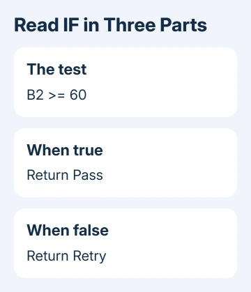
The general pattern is =IF(test,result_when_true,result_when_false). The first part asks a yes-or-no question. The second is what Excel returns when the condition is met; the third is what it returns when it isn't.
Don't type test or result_when_true into your formula. Those words describe the three parts. In the example, the first part compares B2 with 60. The other two contain the text Excel can return, in quotation marks.
Microsoft describes text and numeric results in its IF function reference. The same formula works in Windows and Mac Excel without a special menu.
If entering formulas is unfamiliar, the Excel formula-entry guide explains choosing an output cell and starting with an equals sign.
Choose the comparison that matches your rule
Use = for equal, <> for not equal, > for greater than, and < for less than. Adding an equals sign gives >= or <=, which includes the boundary value.
For an order that qualifies at 100, a test of B2>=100 includes an order of exactly 100. A test of B2>100 doesn't. Decide that rule before writing the formula, especially when it changes a payment or a grade.
A text comparison needs quotation marks around the text being matched. For example, put a status in A2 and enter this in another cell:
=IF(A2="Paid","Complete","Follow up")When A2 contains Paid, the formula returns Complete. With another status, it returns Follow up. The words in quotation marks are text values; A2 remains a reference to the cell that holds your input.
Ordinary IF equality comparisons aren't case-sensitive, so Paid and paid both match. Extra spaces can still change what's in a cell. Check the input if a status looks right but Excel treats the condition as false.
Use straight quotation marks in a formula. Curved quotation marks copied from formatted text can stop Excel accepting it. The punctuation that separates the three parts must also be present.
Return a number or calculation instead of a label
For either result, you can use a number, a cell reference or a calculation. For a shipping example, put an order total in B2 and use:
=IF(B2>=100,0,8)An order of 120 returns 0, and an order of 80 returns 8. These outputs are numbers, so another formula can add them to an order total. Putting quotation marks around a number would make the returned value text instead.
For a made-up 5% discount that starts at 100, use:
=IF(B2>=100,B2*5%,0)With 120 in B2, that returns 6, the discount amount. It doesn't return the final price of 114. Decide whether your result column should contain the discount or the amount due before copying a calculation through a list.
I'd check the result with one small number I can calculate mentally. Excel can accept a formula even when it calculates a different result from the one you intended.
Copy the formula while keeping the right references
Put the other scores in B3, B4 and later rows. Select C2 and drag its fill handle, the small square at the selected cell's corner, down through the corresponding result cells.
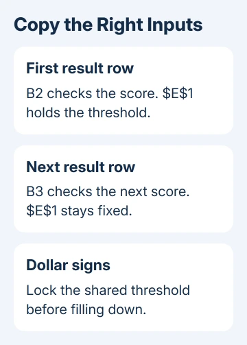
The reference changes as you fill: C3 tests B3, C4 tests B4, and so on. This is a relative reference. Each row gets the same rule applied to its own input.
For a threshold you want to change in one place, put 60 in E1 and use this in C2:
=IF(B2>=$E$1,"Pass","Retry")Dollar signs lock the threshold reference during copying. B2 can become B3 while $E$1 still points to that shared value. Inspect a copied formula to check that its row moved and its threshold didn't.
Don't put the formula in the same cell as the value it tests. That either replaces the input or creates a circular reference, where a calculation depends on its own result.
Handle an empty result and more than one condition
For an empty-looking false result, put two straight quotation marks with nothing between them in the false position. This returns empty text; it doesn't remove the formula or make the cell truly unused.
For a calculation that should wait until an input exists, use the IF not blank examples. That matters when another formula counts or checks those cells: looking empty isn't the same as being unused.
For a calculation that fails after inputs arrive, choose an IFERROR fallback separately from the IF condition.
An AND test requires all its conditions to be true. This example requires both a sufficient score and the word Submitted in C2:
=IF(AND(B2>=60,C2="Submitted"),"Pass","Review")An OR test needs at least one condition to be true. Choose it only when either condition should qualify. Changing AND to OR changes the rule, even if both formulas look similar.
If you need several possible results, you can put one IF inside another. Keep the conditions in a sensible order and test the boundary for each result. Don't add another nested test when a two-result decision already answers the question.
Fix a formula Excel rejects or doesn't calculate
If Excel objects at the commas, your regional settings may use semicolons between the three parts of the formula. The first example would then use this punctuation:
=IF(B2>=60;"Pass";"Retry")Some language versions also use a translated function name.
For #NAME?, inspect spelling and text quotation marks. A cell displaying the formula may be formatted as Text, or Show Formulas may be enabled. Check those settings before changing the test in your formula.
For a wrong result, check the input, operator and copied references. Give a shared workbook's owner one example input, its expected output and the actual formula so they can review the rule.
The Short Version
Use =IF(condition,true_result,false_result), quote text, and test both outcomes. Check boundary values such as 60 in a 60-or-higher rule. When copying, let row inputs change and lock any shared threshold with dollar signs.
Checked November 15, 2026.