How to Divide in Excel: Numbers, Cells and Columns

Excel divides with a forward slash in a formula: type =84/7 into a cell and press Enter to get 12. For numbers already in the worksheet, =A2/B2 uses A2 as the amount and B2 as the divisor.

Keep the equal sign at the beginning. Without it, an entry containing a slash can become a date instead of a calculation.

Calculate using two input cells

Enter 84 in A2 and 7 in B2. Select an unused result cell, such as C2, enter =A2/B2, and confirm with Enter on Windows or Return on Mac. This example returns 12.

Microsoft documents the slash operator in its Excel division instructions. Excel has no ordinary DIVIDE function; the operator performs this calculation.

Status: Excel division, copied references and zero-divisor handling checked November 3, 2026. The displayed results are worked arithmetic examples, not a test workbook.

Changing B2 to 4 makes the example result 21 under normal automatic calculation. This shows why referencing cells is useful: the input can change without rewriting the expression.

The order matters. =B2/A2 calculates the reciprocal of the original ratio, so inspect the formula before changing its number format to make an unexpected answer look different.

In a mixed calculation, group the amount to divide with parentheses. =(84+14)/7 gives 14, while =84+14/7 gives 86 because Excel divides 14 by 7 before adding 84.

Fill down with a divisor on each row

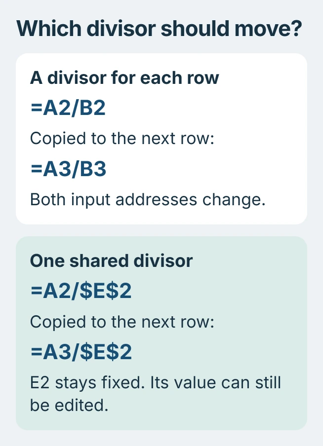
When every record has its own amount in column A and divisor in column B, place =A2/B2 in C2. Copy that formula down the required result rows, using the fill handle at the cell's lower-right corner.

The formula in C3 should become =A3/B3. Check that next row before filling a long list. Both references need to move because each result belongs to its own pair of inputs.

Microsoft says copied formulas can adjust their references in its calculator guide. The Excel formula-copy guide covers other copying and paste choices.

Divide every amount by one fixed cell

For a common divisor, put 7 in E2 and the amounts in A2, A3 and subsequent rows. Enter =A2/$E$2 in B2 and fill downward. The dollar signs keep E2 unchanged as the source row advances.

The next formula is =A3/$E$2. With 84 and 140 as the first two amounts, the results are 12 and 20. Select the second result and inspect its formula bar to check that E2 stayed fixed.

An anchored reference fixes the address during copying; it does not lock the divisor against edits. Changing E2 deliberately should change the calculated ratios that use it.

For the reverse operation, multiply by a shared factor. Use the operation that matches the intended calculation instead of changing references until a result looks plausible.

Correct a zero divisor before hiding its error

Microsoft states that #DIV/0! means the divisor is zero or a referenced divisor cell is empty in its error explanation. Read the cell after the slash first.

Supply the missing value or correct the reference. Do not replace a real zero with an arbitrary number simply to remove the error. The calculation has no valid numeric result until its denominator is appropriate.

For a form waiting for a numeric divisor in B2, this example leaves the result visually blank until B2 contains a nonzero number:

=IF(B2,A2/B2,"")

That blank is a display choice, not a calculated zero. The input still needs attention. Microsoft warns that IFERROR hides other errors too, so avoid wrapping an unverified formula merely to make its cell look clean.

If division works in a fresh sheet but fails in the working file, share a small invented-data example with Microsoft Support. Include the formula, input values and exact error rather than a private workbook.

The Short Version

Use a slash after an equal sign. Let both references move for separate row inputs, or anchor the common divisor with dollar signs. Correct an empty or zero denominator before deciding how unfinished results should appear.