
Excel's IRR can return #DIV/0! when its starting guess leads the calculation into trouble. Try =IRR(A2:A10,-10%) with your real range. A loss can produce a negative return; it shouldn't need to appear as an error.
An error already present in the input cells is a separate cause, so check those if the changed guess doesn't help. Keep your real payments and receipts in the calculation. Replacing the error with zero would hide the problem.
In this guide
1. Give IRR a different starting guess
Select the cell with the formula that returns the error and read it in the formula bar. If it uses only the range, such as =IRR(A2:A10), add the optional second argument:
=IRR(A2:A10,-10%)Use your real range instead of the example. The comma separates the cash flows from the guess; if your Excel uses semicolons between formula arguments, use a semicolon here too.
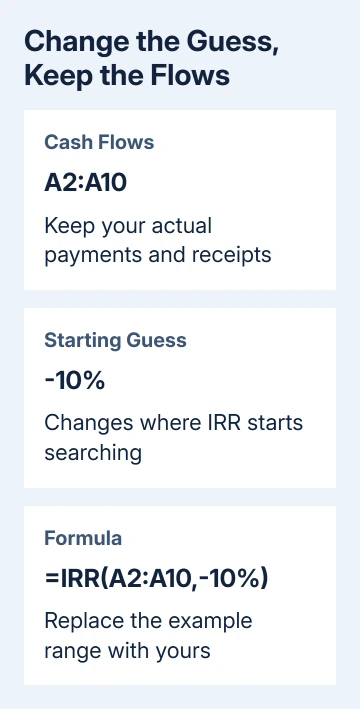
The guess is where the calculation starts searching, not a return you are forcing it to produce. IRR uses 10% when you leave it out, so a different starting point can change whether Excel reaches a result.
Microsoft's IRR instructions recommend changing the guess when the function gives an error or an unexpected result. They describe #NUM! for a failed search; the older owner thread also reports #DIV/0!.
One owner and a second reader in the original IRR discussion confirm the advice fixed their formulas. A negative guess is a useful first attempt, not a rule that every negative return requires -10%.
If the result is a number, format the cell as Percentage so it's readable. If Excel still returns an error, check the actual input cells before trying lots of arbitrary guesses.
2. Look for an error inside the cash-flow range
Inspect every cell included in the IRR formula. A referenced cell showing #DIV/0! because its own formula divides by zero needs repair there. Changing the outer IRR guess won't fix the arithmetic in that input.
Select the first bad input and read its formula. Check whether its divisor is blank or zero, and whether the source it depends on is missing. Correct the underlying value or formula according to what the workbook is meant to calculate.
Duplicate the workbook first, then make your calculation changes in that copy. It's easy to replace the wrong formula while trying to make a financial model display a number.
A temporary =COUNT(A2:A10) in an empty cell can help you compare the number of numeric entries with the periods you expected. If the counts differ, check for blanks, text values, and formulas in the range.
For inputs imported from another workbook, check the financial-model connection before changing the cash flows.
Within a referenced range, IRR skips text entries and blank cells. A payment stored as text can look numeric while Excel leaves it out of the calculation. Check the cell values; a visible currency symbol alone doesn't make them numeric.
Use the Excel number-format checks when the underlying number and its display are confusing. Formatting a cell changes how its value looks, not which cash flow the model should contain.
3. Check signs, order, and the first payment
IRR needs at least one negative value and one positive value. Enter money paid out as negative and money received as positive, Keep the signs consistent with whose money you're tracking: the person's or the project's.
In a later example, changing the guess still failed because the entries were all contributions with the same sign. Include the real ending receipt or value when it belongs in the model, rather than changing signs at random.
For example, an initial payment of 1,000 followed one period later by a receipt of 900 can be entered as -1000 and 900. The return for that single period is -10%. Negative returns are valid results.
Select the formula's range carefully. It should start with the first cash flow and continue through the last one you want to include. If the range misses your initial investment, the result won't answer the question you meant to ask.
Keep the cash flows in their actual time order. IRR treats the first entry as the first period and the remaining numeric entries as successive equal periods. Sorting by amount changes the calculation's meaning.
A zero-payment period needs a numeric zero when that period belongs in a regularly spaced series. A blank cell is ignored, so leaving it blank can make later cash flows occupy the wrong positions in the calculation.
If the signs or range were wrong, correct them and calculate again. If they were already right, move to the timing check rather than changing a real payment merely to make the error disappear.
4. Use XIRR when the payment dates are irregular
IRR assumes regularly spaced periods, such as one month between every entry. If your receipts arrive on uneven dates, use XIRR with both the values and their corresponding dates.
For example, with cash flows in A2:A10 and matching dates in B2:B10, enter:
=XIRR(A2:A10,B2:B10,-10%)Each value needs its matching date. Use actual Excel date values rather than text labels that only look like dates, and keep the rows paired when you edit or sort the data.
This accounts for the actual payment dates; it won't fix every #DIV/0! error. XIRR can also fail to reach a result. It still needs the right inputs, including positive and negative cash flows.
Don't compare a monthly IRR directly with an annual XIRR and assume the different numbers mean one function is broken. IRR's rate belongs to the spacing of its periods; XIRR returns an annual rate.
If the dates and values are right but XIRR returns an error, inspect its own error message and input requirements. Keep the original IRR formula separately until you're sure the new function suits your payment timing.
5. Check a successful result instead of stopping at a number
A changed guess can produce a number that still needs checking. Cash flows that change sign more than once can have more than one possible internal rate of return, so different guesses may lead to different answers.
I'd check those sign changes before treating the first returned percentage as the only answer. A series with an initial outflow, later receipts, and another large outflow needs more care than a simple purchase followed by income.
For regularly spaced flows, compare the result with a net present value calculation. If A2 is the initial cash flow and A3:A10 are later flows, this check should be close to zero at a valid IRR:
=NPV(C2,A3:A10)+A2In this example, C2 holds the calculated rate. Keeping the initial cash flow outside NPV matters because it occurs at the start, while the function discounts the later payments.
Don't wrap IRR in IFERROR(...,0) as a repair. That hides the failure as a 0% return and can make a broken calculation look like a valid result.
For a remaining error, gather the cash flows, relevant dates, formula, Excel version, and guesses tried. Ask a spreadsheet specialist whether the sample has a valid rate and whether more than one answer is possible.
The Short Version
Try a different IRR guess, then check input errors, signs, and period order. Use XIRR for irregular dates. A returned percentage needs checking too, especially when the cash flows change sign more than once.
Checked November 17, 2026.