
SUMIF returning zero or the wrong total usually needs its criteria, number formats or ranges corrected. Check one row that should match before changing the sheet. A #VALUE! error can come from a closed source workbook.
These steps apply to Excel on Windows and Mac. If the cell shows the formula itself, Excel hasn't calculated a total yet. Start with the check that matches what you see in your sheet.
In this guide
1. Check what SUMIF is testing and adding
SUMIF tests cells in one range and adds the corresponding numbers in another. For example, put Apples, Pears and Apples in A2:A4, with 10, 7 and 5 in B2:B4. This formula should return 15:
=SUMIF(A2:A4,"Apples",B2:B4)The first range holds the labels to test. The middle part is the condition to match. The last range holds the amounts to add. Microsoft's SUMIF function reference explains that order.
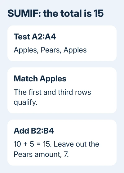
Compare those three parts with your formula. Testing the amount column when you meant to test labels can give a total that doesn't answer your question. Check that the first range holds the labels and the last holds the amounts to add.
If your formula is printed in the cell instead of showing a total, check Formulas > Show Formulas first. If only that cell is affected, change its format from Text to General, then edit the formula and press Enter again.
Look for an apostrophe before the equals sign too. That tells Excel to treat the entry as text. Remove it only from a cell that should contain a formula, rather than changing an entire column of intentionally stored identifiers.
2. Write criteria with the correct quotes and operators
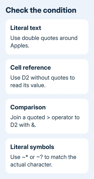
Text conditions need double quotation marks. Put double quotes around a literal label such as Apples. Use D2 without quotes to read the label from D2. With quotes, Excel looks for the text D2 instead of the label in that cell.
For a numeric comparison, keep the comparison symbol inside quotes. This example adds numbers greater than 100 from B2:B20:
=SUMIF(B2:B20,">100")When the limit comes from another cell, join the comparison symbol to that cell reference with an ampersand (&). With the limit in D2, use:
=SUMIF(B2:B20,">"&D2)Check your regional list separator if Excel rejects the formula before calculating. Some installations use semicolons where these examples show commas. Keep the separator consistent rather than adding both.
If correcting the condition gives you the expected total, SUMIF wasn't matching the rows you wanted. If the condition is now right but the total remains zero, inspect one of the amounts next.
3. Convert amounts that are stored as text
Imported amounts can look numeric while Excel stores them as text. A currency symbol or right-aligned amount doesn't tell you how Excel stored it. In an empty cell, test a suspect amount with =ISNUMBER(B2).
TRUE means B2 contains a number. FALSE means it isn't a numeric value for that test. If an amount is text, select those amounts and choose the warning button's Convert to Number command when offered.
Changing the display format to Number alone won't turn text into numbers. If the warning control isn't available, Microsoft's text-to-number conversion steps give other methods.
For imported dates, use the Excel date-conversion checks before applying a date condition. A date that only looks correct can still be text, which changes how the comparison behaves.
I'd convert a small sample and check the total before changing a large import. Account codes and postal codes can intentionally be text; converting them can remove leading zeros that matter.
4. Align both ranges and lock them before filling
Use the same rows and shape for the tested range and the added range. For labels in A2:A20, amounts for those same records should be B2:B20. A range starting on row 3 adds an amount from the next record instead.
SUMIF can accept different-sized ranges without reporting the mismatch. It starts at the first cell in sum_range, then adds from an area with the same row and column count as the tested range. The total can look right even when it's wrong.
For example, avoid =SUMIF(A2:A20,D2,B2:B10). Write the full intended amount range as B2:B20 so the formula shows which rows it will add, rather than depending on Excel extending the range.
If the first total works but later copied formulas fail, inspect their references. Use dollar signs to keep the data ranges fixed while letting the reference to the condition cell change:
=SUMIF($A$2:$A$20,D2,$B$2:$B$20)Filling down changes D2 to D3, while the two data ranges stay put. The same moving-reference mistake can affect VLOOKUP results after filling down, so check neighboring formulas if several totals shifted together.
5. Check spaces, wildcards and multiple conditions
Compare a label that should match with the criteria cell. Leading or trailing spaces can make visually similar text different. Use TRIM in a spare column to clean ordinary extra spaces, then check the result before replacing source labels.
In criteria, an asterisk matches a sequence of characters; a question mark stands for one character. The pattern Apple* matches Apple and Apples. For the actual symbols, put ~* or ~? inside your quoted condition.
SUMIF handles one condition. For a total that must match both a product and a region, use SUMIFS instead. SUMIFS takes the amounts to add first, then each range to check and its condition.
In SUMIFS, each range must match the others in row count and column count. Don't copy a SUMIF formula, add another condition at the end and assume the argument order stayed the same. Review each range against the rows in the source data.
6. Open external workbooks for a #VALUE! error
If the formula refers to a separate workbook, open that source workbook and recalculate. SUMIF and SUMIFS can return #VALUE! when their referenced workbook is closed. Use Formulas > Calculate Now after opening it.
The SUMIF error guidance also identifies criteria strings longer than 255 characters as a source of incorrect results. Prefer a shorter matching key where possible.
If the result still fails, copy a few nonprivate source rows and the exact formula into a small sample workbook. Give that example to your spreadsheet owner or Microsoft Support, with the expected total calculated from those rows.
With a small sample, you can show exactly where a range or condition goes wrong. Avoid wrapping the formula in IFERROR until the actual total is right; replacing an error with zero can leave a broken calculation looking finished.
The Short Version
Check the criteria syntax, convert text amounts and align the tested and added rows. Lock ranges before filling down. Use SUMIFS for multiple conditions, and open a referenced source workbook when SUMIF returns #VALUE!.
Checked November 13, 2026.