How to Round Up in Excel With ROUNDUP

To round up in Excel, enter =ROUNDUP(A2,0) in another cell, replacing A2 with the cell holding your number. That turns a positive value such as 6.2 into 7; use 2 instead of 0 when you need two decimal places.

ROUNDUP moves away from zero, so a negative number becomes more negative. For boxes or seats, decide whether you need a whole number or a particular pack size before choosing the formula.

Put the rounded result in a separate cell

Keep the original number in A2 and click B2 for the result. Type =ROUNDUP(A2,0), then press Enter. With 6.2 in A2, B2 should display 7. An existing whole number such as 6 stays 6.

Microsoft's ROUNDUP reference explains both parts of the formula. The first tells Excel which number to round; the second tells it where to round.

Using a separate column lets you compare the result with the original number. Once the formula is right, change A2 and watch B2 update. This also helps you spot a formula pointing at the wrong row.

Typing =ROUNDUP(6.2,0) works too, but that formula always uses 6.2. Referring to A2 is more useful when you'll change the original number later. Leave the equals sign at the start so Excel treats it as a calculation.

Choose the digit setting your calculation needs

The second part of the formula is called num_digits. It tells Excel where to round the number, not how much to add.

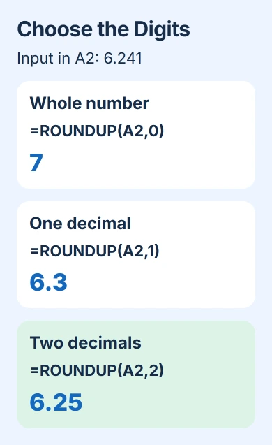
For an input of 6.241, these formulas produce different results:

Formula	Result	Use it for
=ROUNDUP(A2,0)	7	A whole item
=ROUNDUP(A2,1)	6.3	One decimal place
=ROUNDUP(A2,2)	6.25	Two decimal places

A negative digit setting rounds to the left of the decimal point. With 142 in A2, =ROUNDUP(A2,-1) returns 150, while =ROUNDUP(A2,-2) returns 200. Those settings work in tens and hundreds.

Choose the setting to suit the job. Rounding a measurement to one decimal place is different from working out how many whole containers you need.

Use whole packs when a decimal count isn't useful

Suppose a job needs 25 items and each box holds 12. Enter 25 in A2 and 12 in B2. The formula =ROUNDUP(A2/B2,0) returns 3, which is the number of boxes to order.

Two boxes only hold 24 items, so rounding the division to its nearest whole number would leave you short. I'd keep the required quantity and pack size in separate cells so the reason for the result stays visible.

To find how many items those boxes supply, use =ROUNDUP(A2/B2,0)*B2. That returns 36 items. Label the result column clearly so someone reading the sheet doesn't mistake items for boxes.

For a positive quantity, you can also use =CEILING.MATH(A2,12). This rounds to a multiple of 12 and returns 36. The CEILING.MATH instructions explain how it handles multiples and negative numbers.

Don't substitute ROUNDUP(A2,12) for either formula. The 12 sets the number of decimal places; it doesn't mean packs of 12. The formulas look similar, but they give very different results.

Check negative values before copying the formula

ROUNDUP's direction matters for refunds, debts and temperatures. =ROUNDUP(-6.2,0) returns -7. That moves farther from zero, even though -7 is a smaller number than -6.2.

If you need to round toward a greater number, =CEILING.MATH(-6.2) returns -6 with its default settings. Decide which result you need before using a formula in a column with positive and negative values.

Try one positive number, one negative number and one exact whole number. These three examples make the rule easier to see than a column of similar positive values. Keep them separate from your working data.

Ordinary ROUND chooses the nearest result for the digit setting you give it. It doesn't always round away from zero. Use it when you need the nearest value, rather than another whole item for every fraction.

Fill the formula down and check its references

After checking B2, select it and the cells you want to fill in that column. Use Home > Fill > Down, or press Ctrl+D in Windows Excel. The fill-down procedure copies the formula into the selected cells.

After filling down, B3 should refer to A3, not A2. Click a result farther down the column, then read the calculation in the formula bar. A repeated result can come from a formula still pointing at the first input.

If every row uses a pack size stored in D1, use =ROUNDUP(A2/$D$1,0). The dollar signs keep D1 fixed while A2 changes as you fill down. Keep that shared pack size separate from the quantities that change in each row.

For a report with several numeric columns, decide when to calculate each row's total. Rounding every line and then adding can give a different answer from adding first and rounding once.

Fix a result that only looks rounded

Changing the displayed decimals doesn't usually create the rounded value needed by another formula. If Excel seems to round without ROUNDUP, check the displayed versus stored digits before changing the calculation.

If Excel rejects a copied formula, check the separator your copy uses. Some installations use semicolons, so =ROUNDUP(A2;0) is the same formula. Look at a working formula in your workbook to see which separator to use.

If you still can't explain a result, keep the original number, complete formula and expected answer together. Show that small example to the workbook's author or Excel Support. It's easier to check than a total without its inputs.

The Short Version

Use ROUNDUP with 0 for whole items, positive digits for decimals, or negative digits for tens and hundreds. For packs, round the division or use CEILING.MATH. Check negative inputs and copied references before relying on the column.

Checked November 5, 2026.