How to Add a Filter in Excel and Show Matching Rows

An Excel filter hides nonmatching records while keeping them in the worksheet. Select the data, including its headings, then choose Data > Filter. Use a column heading's control to choose which values remain visible.

Filtering is useful when a long list contains several regions, statuses or dates and only one group needs attention. It does not sort the records or delete the ones that disappear.

Give the filter the complete list

Identify the first heading, final column and last record before applying the filter. Select that rectangular range so the filter covers every field belonging to each record, including data after any gaps.

Microsoft documents Data > Filter for ordinary ranges in its Excel filtering instructions. The heading controls appear once filtering is enabled.

Status: Excel range, table and filter-clearing instructions checked November 3, 2026. The example uses invented records; no workbook was changed.

For a simple continuous list, selecting a cell inside it also works. Explicitly selecting the full range makes its intended boundaries easier to check when the sheet contains several separate blocks.

If the headings already have controls because the data is an Excel table, use those existing controls. Applying the Filter command again can switch them off.

Choose a value, then narrow another column

In Excel for Windows or the web, open the desired heading's filter menu. Clear Select All, select the values to display, and choose OK. The other rows disappear from view without being removed from the file.

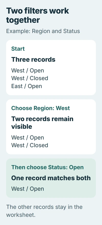
For example, keep West in a Region column. Then open a Status column and keep Open. The remaining records must satisfy both choices: West region and Open status.

Microsoft says additional column filters narrow the current result. A value absent from the second menu may belong only to records already hidden by the first filter.

For a numeric cutoff, use Number Filters, choose a comparison such as Greater Than, and enter the cutoff. A date column offers date-specific choices; a text column offers comparisons such as Contains.

On Excel for Mac, use Data > Filter, open the heading control and choose the comparison under Filter > Choose One. Enter its value and apply the condition shown in that menu.

If the goal is alphabetical order instead, sort the records by the name field. A filter reduces what is visible; sorting changes the order of the records.

Use a table for a list that will keep growing

Select the complete data block, choose Home > Format as Table, and pick a style. In the dialog, verify the range and select My table has headers when the first row contains field names.

The table-creation procedure adds filter controls to the headings automatically. Confirm the table contains the final record before choosing a filter.

A colored row alone is not an Excel table. Formatting cells with a fill color does not establish the table's boundaries or add its controls.

Keep the heading row separate from the data. A first record accidentally treated as a heading will not be filtered alongside the other records.

Clear the conditions to bring records back

Open the filtered column's menu and choose Clear Filter From followed by its heading name. This clears that column's condition. Conditions on other columns still apply.

In Windows desktop Excel, Data > Clear clears the applied filters across the range. Microsoft states in its filter-removal guide that Data > Filter removes filtering altogether.

After editing data or adding records, use Data > Reapply in desktop Excel to apply the current conditions again. Check that new records belong to the filtered range or table before expecting them to appear.

If rows remain missing after all conditions are cleared, check whether they were hidden manually in Excel. Clearing a filter and unhiding rows address different causes.

Check the range when results look incomplete

Confirm that the filter includes the missing records and no second column has an active condition. Compare displayed values with their cell contents; imported numbers stored as text can change the available filter choices.

For an unavailable Filter command, check editing permission and worksheet protection with the workbook owner. If the same problem occurs in a new unprotected file, report the Excel edition and exact behavior to Microsoft Support.

The Short Version

Enable filtering on the complete list, choose values in a heading menu and apply additional conditions only when needed. Clear conditions to restore the records, and verify the range whenever new entries seem missing.