
Excel can color a cell or row when another cell meets a condition. Create a formula-based rule and lock its column reference with a dollar sign. For example, a Done status in column D can trigger a highlight across that task's row.
The selected range controls what gets colored; the formula controls what Excel checks. Keeping those two jobs separate prevents the common problem where the wrong row changes color or every row follows one status cell.
In this guide
Select the cells that should change color
Suppose columns A through D contain a task list, with headings in row 1 and a status in column D. To color each completed task's whole row, select A2:D20. Leave the heading row out of the selection.
For an exact selection, use the Name Box just left of the formula input area, enter A2:D20, and press Enter. The highlighted block should cover the task rows, starting at row 2.
To color only the task name, select A2:A20 instead. The formula can still check column D even though the cells receiving the color are in column A. The tested cell doesn't have to be part of the colored range.
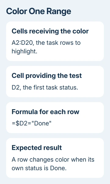
The ordinary Excel highlighting controls apply a fixed fill or a built-in value rule. Use the formula method when the value in another column should control the color.
Create the formula rule in Excel for Windows
With the target range selected, open Home > Conditional Formatting > New Rule. Choose Use a formula to determine which cells to format. Enter this expression in the formula box:
=$D2="Done"Select Format, open Fill, and choose a readable background color. Select OK to accept the appearance, then OK again to create the rule. Rows with Done in column D should turn that color.
Microsoft says the test must return TRUE or FALSE in its formula-based formatting instructions. The formula checks whether the condition is true; it doesn't change the values in your cells.
Try a completed status in D2 and a different status in D3. Only the matching row should change. Then change D2 to the other status and check that the conditional color disappears from that row.
A formula result that changes while its color stays stale in Excel 2010 needs the worksheet refresh checks, including its formatting calculation property.
Keep the first row in the formula aligned with the first row in the selected range. A range starting at A2 needs a check based on D2. Starting the test at D3 shifts the decision one row away from the task it belongs to.
Lock the column without locking every row
The dollar sign in $D2 fixes the reference to column D. The row number has no dollar sign, so Excel checks D2 for the first row, D3 for the next row, and so on.
Using $D$2 would lock both parts. Every row in the formatted range would then depend on the one cell D2. That is useful for one master switch, but wrong when each task has its own status.
With D2 and no dollar signs, both the column and row can shift as Excel checks each cell in the range. When coloring A through D, that can make neighboring cells check different status columns.
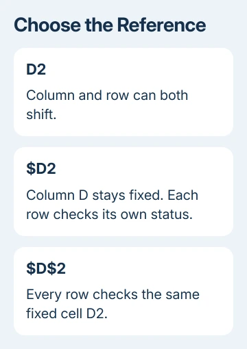
I'd check the dollar signs before rebuilding a rule. If every row turns the same color together, a locked row is a more useful place to look than the fill palette.
For one fixed threshold, locking both parts can be exactly right. To color B2:B20 when each amount exceeds the limit in F1, use =B2>$F$1. Each amount changes by row while F1 remains the shared limit.
Use a number or combine two conditions
A comparison with another cell can be numeric. If column B holds the amounts and column C holds their targets, select B2:B20 and use =B2>C2. Only amounts greater than their same-row targets should receive the chosen format.
To color the whole row for that comparison, select A2:D20 and use =$B2>$C2. Locking both column letters keeps each colored cell in a row checking the same pair of amounts.
For two requirements, combine them with AND. This example matches rows with a Done status and a column C amount greater than 100. Both tests must be true:
=AND($D2="Done",$C2>100)Check a complicated condition by entering its formula in a spare cell. TRUE should appear for a row you expect to color. If Excel displays the expression instead of evaluating it, repair Excel's formula display.
Find the formula controls on Mac or the web
In Excel for Mac, select the target cells and open Home > Conditional Formatting > New Rule. In Style, choose Classic, then choose Use a formula to determine which cells to format in the rule list.
Enter the same formula. Under Format with, choose the custom format option, select the required fill, and accept the dialogs. The Mac layout differs from Windows, but the reference locks work the same way.
For the browser edition, choose Home > Conditional Formatting and create a rule in its pane. Set Rule Type to Formula, enter the condition, choose the appearance and use the pane's apply control to save the rule.
The browser pane and the desktop dialog aren't identical. Use the named Formula rule type in the browser rather than searching for a Mac-only Classic list. Keep the selected range and reference row the same across versions.
Correct a rule that colors the wrong cells
Open Home > Conditional Formatting > Manage Rules and find your rule. In Windows, show rules for the whole worksheet if you can't see it for the selected cells. Check both the formula and Applies to.
For the task example, keep the Done condition from the first example, with the range set to =$A$2:$D$20. A correct formula applied only to A2 can't color the rest of the table.
Check the status cell for unwanted spaces if a word looks right but doesn't trigger the rule. Check the other formatting rules too. If several rules set a fill color for the same cell, their priority can decide the color you see.
A different fault makes cell alignment fail when a rule applies, even while the ribbon still shows Center.
If workbook protection or sharing restrictions limit editing, ask the owner to review the rule. Send the formula, target range and two example rows: one that should match and one that shouldn't. Those examples help them see what's wrong.
The Short Version
Choose the target range, create a Formula rule, and check the other cell with the right reference locks. Use $D2 for a status column that changes by row, and $D$2 when every row must depend on one fixed cell.
Checked November 13, 2026.