

New data columns won't appear in PivotTable Fields while the source still ends at the old column. Select the extra columns as part of the source, then refresh. Saving the workbook alone doesn't expand its source.
A formula column can be a source field too. Check the range and headers before replacing calculations with fixed numbers. If the whole Fields pane has disappeared, restore it first; that's different from one missing field.
In this guide
1. Check the source boundary, then refresh
Select a cell belonging to the PivotTable. For the current Windows desktop version of Excel, choose PivotTable Analyze > Change Data Source. The dialog shows the table name or cell range feeding that report.
For Excel 2007 and 2010, choose PivotTable Tools > Options > Change Data Source. On current Excel for Mac, select the report and look under its Analyze tab for Change Data Source.
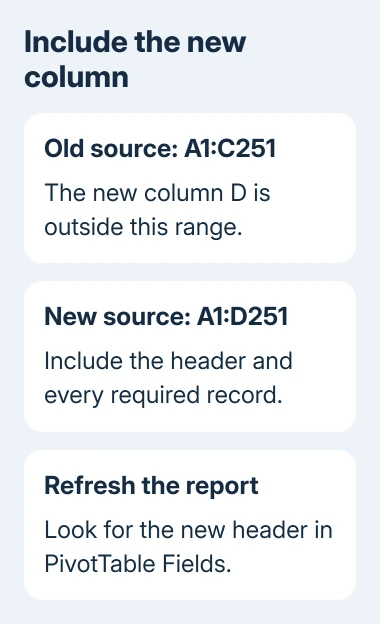
Compare the last column in the dialog with the new column's position on the data sheet. For example, a source of A1:C251 cannot include a new column D. Change the selection to A1:D251 if that describes your actual data.
Include the header row and every required record, then select OK. Right-click inside the PivotTable and choose Refresh. Look for the new header in the Fields list before changing the arrangement of the report.
Microsoft's source-data instructions explain the range change. If the source structure has changed substantially, including the number of columns, they also recommend considering a new PivotTable.
Once the field appears, drag it into the area you need. Compare its results against the source records. Being listed confirms that Excel sees the column; it doesn't mean the report is already using it.
2. Restore a hidden list or find the renamed field
Click the report again if PivotTable Fields isn't visible. In desktop Excel, choose PivotTable Analyze > Field List. The pane belongs to the selected report, so clicking ordinary worksheet cells can hide the relevant ribbon controls.
If the pane is present, check the source header's exact wording. The field uses that heading as its name, rather than the worksheet column letter. A column added in position N won't appear as N unless its header actually says that.
Give source columns distinct headings. Two columns shouldn't use the same name for different information. One owner in the missing-fields discussion traced the problem to duplicate labels.
After correcting headers, refresh the report and inspect the list again. Don't drag an old field into the report simply because its name looks similar. Check the source values so the report summarizes the intended column.
If the heading is unique and inside the selected range but still absent, check whether the source uses a named range or an Excel Table. A name can make it harder to spot that the range still stops at the old column.
3. Expand the named range or the Excel Table itself
A source such as SalesData is a name, not a promise to include the whole worksheet. In desktop Excel, open Formulas > Name Manager, select that name, and inspect Refers to.
If the definition ends before the new column, edit it to include the complete data and headers. Keep the original sheet reference intact. Return to the PivotTable, refresh it, and check whether the missing heading appears.
The accepted answer used a named range. Its menu path was for an older interface; current desktop Excel has Name Manager. Edit the name the report actually uses, rather than another name elsewhere in the workbook.
For an Excel Table, click inside the source table and inspect its highlighted boundary. A column separated by a blank column can sit outside it. On Windows, Table Design > Resize Table lets you include the required adjacent data.
For future additions, using an Excel Table as the source helps include new columns in the field list. Refresh after adding them. Keep calculations and their headers inside that source table.
The PivotTable creation walkthrough explains how fields become rows, columns and totals. Return to that arrangement only after the new field is available to select.
4. Keep formula columns and check the report's source type
A worksheet column containing formulas doesn't need to become fixed values just to qualify as a PivotTable field. Check its header and source boundary first. Replacing formulas removes their ability to recalculate when the inputs change.
If the field appears but the totals are wrong, you're dealing with a different problem. Check whether the calculated results are numeric and whether Values uses Sum or Count. A visible field and a missing field need different corrections.
If the date field is present but grouping fails, check for dates stored as text before changing the source columns again.
For a report built from the Workbook Data Model, you can't change the source range in the same way. The Data Model is a separate collection of tables used by the workbook, rather than the cells currently selected on screen.
Have the workbook's maintainer check the model or query that supplies that table. A new worksheet column won't become a model field just because it sits beside data that was imported earlier.
A report that fails only when opened from SharePoint needs a local-copy refresh comparison rather than another field arrangement.
For a browser workbook missing the source controls, use Open in Desktop App if available. Check the actual source there instead of rebuilding a complicated report with a guessed range.
5. Rebuild a test report if the expanded source still fails
Save a separate workbook copy, select the complete current source and choose Insert > PivotTable. Put the test report on a new worksheet. Check its Fields list before adding any totals or formatting.
If the new report sees the column, compare its source with the old report's source. Rebuild the old layout in the test report only after checking the totals. Leave the original report available until the replacement is correct.
Closing Excel helped some owners, but the original asker later reported the missing-column problem again. I'd check the range before relying on a restart. The range controls which data the report actually reads.
If a fresh report still misses the field, give Microsoft Support a harmless workbook sample, both source definitions and the missing header. Mention whether the source is a range, Table, query or Data Model.
For a report that sees all fields but puts them in the wrong order, the PivotTable sorting checks address that separate layout problem.
The Short Version
Expand the actual source, keep distinct headers and refresh. Inspect named-range and Table boundaries before changing formulas. Try a fresh report after major source changes; check model-based reports at their model or query.
Checked November 16, 2026.
 If you have any business, I can build it online